SQS: Fusing Pruning and Quantization into One Bayesian Learning — Where Spike-and-Slab Meets GMM
TL;DR — Doing pruning and low-bit quantization separately leaves redundancy on the table. SQS couples a spike-and-slab prior with a Gaussian mixture model (GMM) into a single variational learning scheme, achieving higher compression at the same bit-width and lower accuracy loss at the same compression ratio.
Core Idea
The two most widely used techniques for making deep learning models lightweight are pruning (zeroing out unimportant weights to reduce the parameter count) and quantization (converting weights from high precision such as FP32 to low bit-widths such as INT8/INT4). Applied sequentially, however, they fail to see the redundancy each stage leaves behind, forcing overly conservative compression ratios to preserve target accuracy.
The question SQS ( Sparse Quantized Sub-distribution) poses is simple.
What if we optimize pruning and quantization simultaneously?
The answer this paper gives is Bayesian variational inference. A single posterior learns both which weights to remove and what low-bit values the surviving weights should take. And the shape of that posterior is the paper’s signature: spike-and-slab + GMM.
Background: The Problem They Set Out to Solve
The classical problem in model compression is distributional shift. Pruning or quantization distorts the original weight distribution and causes performance degradation. To avoid it:
- Pruning has advanced through the OBS/OBC family (ExactOBS, PLATON, etc.), which measure weight importance with second-order information, and
- Quantization has seen the rise of continuous-mapping methods that approximate the weight distribution with a GMM, avoiding the training instability caused by the pseudo-gradients of the straight-through estimator (STE).
DGMS in particular auto-learns the quantization set with a GMM, but it cannot enforce sparsity during training. This problem shows up most dramatically in LLMs. Compressing Llama3.2-1B and Qwen2.5-0.5B, DGMS collapsed accuracy by 46.67% and 50.80%, respectively. The reason is that self-attention weights follow a long-tail distribution rather than a normal one, so the GMM fails to capture the large-magnitude outlier weights.
In short, the research gap this paper targets boils down to one thing.
There is no method that unifies pruning and quantization into one while preserving high compression ratios and minimizing performance degradation.
New Approach: SQS (Sparse Quantized Sub-distribution)
The crux of SQS is defining the variational posterior as a spike-and-slab + GMM. This structure naturally houses both goals—pruning and quantization—inside a single distribution.
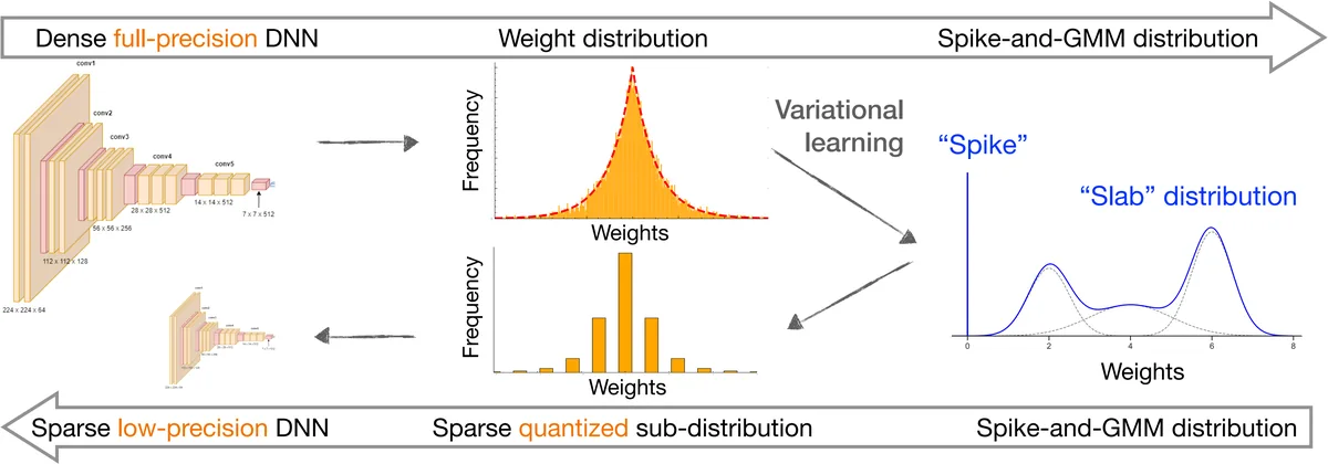
The prior is set to a spike-and-slab. Each weight $\theta_i$ is defined together with a binary indicator $\gamma_i$ indicating whether it is preserved, as follows.
$$\pi(\tilde{\theta}_i) = \lambda\, \mathcal{N}(0, \sigma_0^2) + (1-\lambda)\, \delta_0$$Here $\delta_0$ is a point mass at 0 (the spike), $\mathcal{N}(0,\sigma_0^2)$ is the continuous distribution (the slab), and $\lambda$ is the prior probability of keeping a weight. For example, if the target sparsity is 90%, setting $\lambda=0.1$ means each weight is removed with 90% probability.
The variational posterior extends the slab into a GMM with $K$ components.
$$q(\tilde{\theta}_i) = \tilde{\lambda}_i \sum_{k=1}^{K} \phi_k(\theta_i)\, \mathcal{N}(\mu_k, \sigma^2_k) + (1-\tilde{\lambda}_i)\, \delta_0$$- $\tilde{\lambda}_i$: variational probability of keeping weight $\theta_i$ (low values mean the weight is pruned)
- $\{\mu_k, \sigma^2_k, \pi_k\}_{k=1}^K$: a learnable quantization codebook (each $\mu_k$ is itself a low-bit value)
- $\phi_k(\theta_i)$: softmax mixture weights sharpened by temperature $\tau$ — they converge to a single dominant component as $\tau \to 0$
In this structure, the spike ($\delta_0$) handles pruning and the slab (GMM) handles quantization. The two tasks are jointly optimized in a single parameter space.
ELBO and Its Approximation
The training objective is the negative ELBO, and the catch is that the KL divergence between $q(\tilde{\theta}_i)$ and the spike-and-slab prior has no closed form. The authors derive an approximate objective that plugs in the per-coordinate posterior mean $\theta^{\mathrm{avg}}=\mathbb{E}_{q}[\tilde{\theta}]$.
$$\Omega_{\text{apx}} = -\log p(D \mid \theta^{\mathrm{avg}}) + \sum_{i=1}^{T} \mathrm{KL}\!\big(\mathrm{Bern}(\tilde{\lambda}_i) \,\|\, \mathrm{Bern}(\lambda)\big) + \sum_{i=1}^{T} \tilde{\lambda}_i\, \mathrm{KL}\!\big(\mathcal{N}(\mu_{k_i^*},\sigma^2_{k_i^*}) \,\|\, \mathcal{N}(0,\sigma_0^2)\big)$$- First term: evaluates the likelihood at the full parameter vector $\theta^{\mathrm{avg}}$ (plug-in approximation)
- Second term: regularizes each weight’s keep probability $\tilde{\lambda}_i$ toward the prior $\lambda$ (induces sparsity)
- Third term: regularizes the selected component $k_i^*=\arg\max_k \phi_k(\theta_i)$ toward the prior slab
Theoretically, under mild conditions, SQS’s variational posterior is shown to converge to the true regression function in Hellinger distance. The convergence rate decomposes into three terms — the statistical estimation error $\varepsilon_n^*$, the variational error $r_n^*$, and the approximation error $\xi_n^*$ — of which the first two vanish as $n\to\infty$.
How It Works: A Concrete Example
To make the idea concrete, suppose a single layer has 6 weights.
$$\theta = [0.92,\ -0.81,\ 0.07,\ 0.04,\ -0.85,\ 0.90]$$With a GMM of $K=2$ components (i.e., 1 bit, $\log_2 2 = 1$), the trained codebook would converge to roughly $\mu_1 \approx 0.88$ and $\mu_2 \approx -0.83$.
Step 1 — Quantization (slab): For each weight, the mixture weight $\phi_k(\theta_i)$ is computed, assigning $+0.92$ to $\mu_1$ and $-0.81$ to $\mu_2$. Large-magnitude weights are “snapped” onto codebook values.
Step 2 — Pruning (spike): In contrast, negligible weights such as $0.07$ and $0.04$ learn a low keep probability $\tilde{\lambda}_i$ and eventually fall into $\delta_0$, becoming 0.
Result:
$$\tilde{\theta} = [0.88,\ -0.83,\ 0,\ 0,\ -0.83,\ 0.88]$$| Item | Original | After compression |
|---|---|---|
| Storage bits | $6 \times 32 = 192$ bit | $4 \times 1$ (index) $+ 2 \times 32$ (codebook) $= 68$ bit |
| Non-zero weights | 6 | 4 (33% removed) |
The compression-ratio formula generalizes this calculation.
$$\text{Compression rate} = \frac{32 \times \text{original number of weights}}{\log_2 K \times \text{number of non-zero weights} + 32 \times K}$$In real models, the number of non-zero weights dominates, so the $32\times K$ term in the denominator (codebook storage) becomes negligible and index storage dominates.
Three “Secret Weapons”
SQS’s performance comes from three design choices.
Spike-and-slab prior. What if we replaced it with a Gaussian prior? On ResNet-18/CIFAR-100 with $K=16$, 4-bit, at a 20% non-zero ratio (40× compression), the Gaussian prior collapsed accuracy by 44.04%, whereas spike-and-slab lost only 5.59%. The point mass $\delta_0$ effectively induces posterior sparsity at high sparsity levels.
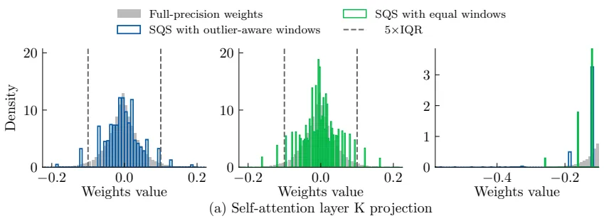
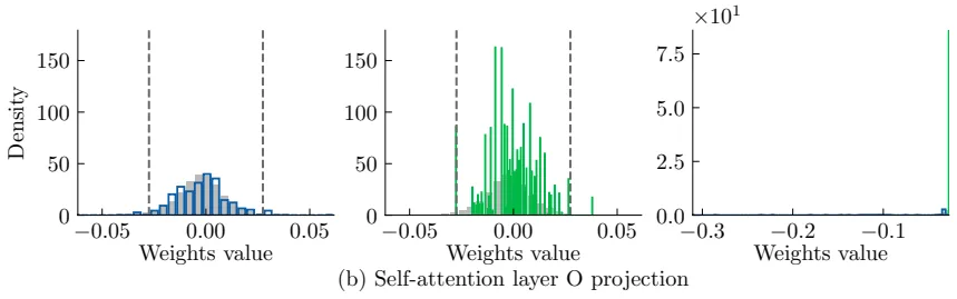
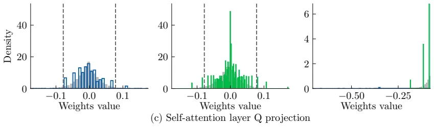
Outlier-aware windowing. LLM weights are long-tailed, so dividing them into uniform-width windows smears large values across wide bins and quantizes them coarsely. The authors split the distribution into 4 windows with a 5×IQR rule to preserve both tails separately. On Qwen2.5-0.5B/SST-2 under identical conditions (6-bit, 50% non-zero), accuracy loss improved from 5.40% with uniform windows to 2.46% with outlier-aware windows, a 2.94 percentage-point gain.
Bayesian averaging. At inference, $M$ weight samples are drawn from the posterior and their predictions are averaged. This always yields lower loss than the greedy approach of using only the single most likely codebook value. Accuracy loss drops from 3.76% at $M{=}1$ to 2.86% at $M{=}5$ and 2.63% at $M{=}50$, with most of the gain coming from a small number of samples (default $M{=}4$).
The effect of outlier-aware windowing is clear in the figures below. Looking at the K, O, and Q projection weight distributions of Llama3.2-1B self-attention, the outlier-aware windows (left) preserve the full precision distribution far better than uniform windows (center), with the difference most pronounced in the left-tail region (right).
Performance Validation: Key Results
Two metrics are evaluated: compression ratio and performance loss (accuracy or F1 loss). All methods are initialized from the same full-precision pretrained model and compressed under the same hyperparameters with a 24-hour cap.
ResNet (CIFAR-10)
| Model | Method | Bits | Non-zero ratio | Compression | Top-1 accuracy loss | |—|—:|—:|—:|—:| | ResNet-20 | DGMS | 2 | 56% | 29× | 0.87% | | ResNet-20 | SQS | 2 | 50% | 32× | 1.47% | | ResNet-32 | TTQ | 2 | 100% | 16× | 1.90% | | ResNet-32 | SQS | 2 | 50% | 32× | 1.29% | | ResNet-56 | TTQ | 2 | 100% | 16× | 1.06% | | ResNet-56 | SQS | 2 | 50% | 32× | 0.84% |
On ResNet-56, SQS achieves 32× compression while holding accuracy loss to 0.84%. At the same 2 bits, that is twice the compression of quantization-only TTQ (16×) with less loss.
BERT-base (SQuAD v1.1)
| Method | Compression type | Bits | Compression | F1 loss | |—|—:|—:|—:| | PLATON | P | 32 | 5× | 2.20 | | GPTQ | Q | 3 | 11× | 2.51 | | OBC | P+Q | 4 | 16× | 2.33 | | SQS | P+Q | 4 | 32× | 1.66 |
SQS records twice the compression of OBC, which combines pruning and quantization, with a smaller F1 loss.
Llama3.2-1B / Qwen2.5-0.5B (SST-2)
| Model | Method | Bits | Non-zero ratio | Compression | Top-1 accuracy loss | |—|—:|—:|—:|—:| | Llama3.2-1B | AWQ | 4 | 100% | 8× | 0.46% | | Llama3.2-1B | DGMS | 6 | 82% | 7× | 46.67% | | Llama3.2-1B | SQS | 6 | 25% | 21× | 1.48% | | Qwen2.5-0.5B | AWQ | 4 | 100% | 8× | 1.54% | | Qwen2.5-0.5B | DGMS | 6 | 34% | 16× | 50.80% | | Qwen2.5-0.5B | SQS | 6 | 50% | 11× | 2.46% |
The most striking result on LLMs is the collapse of DGMS. At the same 6 bits, while DGMS suffers a 46.67%–50.80% accuracy crash, SQS achieves 21×–11× compression with only 1.48%–2.46% loss. AWQ shows even lower loss, but it is quantization-only (no pruning), so its compression stays at 8×.
Comparison with Bayesian Bits
Compared against Bayesian Bits, a representative joint-compression method that places gates on a uniform grid, on ResNet-56/CIFAR-10, SQS records 17.0× compression with 0.84% loss at 2-bit/50% non-zero, beating Bayesian Bits’ 13.5× compression and 6.79% loss. Because SQS learns the codebook values themselves as GMM means, it produces a non-uniform codebook and can control sparsity more precisely than gate-based methods.
Our Take: Strengths, Limitations, and Why This Matters
Strengths
- Genuinely unified. While most joint-compression methods amount to chaining two stages, in SQS a single posterior optimizes both objectives simultaneously. It is a rare case that also comes with a theoretical convergence guarantee.
- Robust quantization. Using the GMM as a vehicle for posterior inference rather than plain clustering enables Bayesian averaging, which buys robustness to quantization noise. This is the decisive difference from DGMS.
- Tackles the LLM long-tail problem head-on. Outlier-aware windowing shares the same motivation as outlier-preserving methods like AWQ, while operating in a setting coupled with pruning.
Limitations
- Task adaptation required. In the LLM experiments, the base model is compressed after being fine-tuned on SST-2. Skipping this step degrades performance substantially. In other words, the reported numbers reflect compression of a task-adapted model, not preservation of general capabilities. Performance under distribution shift or on unrelated tasks is not validated.
- Narrow theoretical scope. The convergence proof is limited to regression problems and fully-connected networks. Transformers and classification settings are not covered.
- Inference latency. Since Bayesian averaging uses multiple samples, latency can increase relative to a single compressed model. The accuracy–latency trade-off needs to be measured on target hardware.
- Extra optimization cost. Retraining after pretraining increases training time and energy before deployment. The paper explicitly acknowledges this.
Why It Matters
The value of this work lies in giving a rigorous Bayesian framework and convergence guarantees to the common wisdom that combining pruning and quantization works better anyway. Especially now that on-device LLM deployment has become a practical requirement, achieving 21× compression at 1.48% loss substantively eases the old tension between compression ratio and performance.
What’s Next?: The Road Ahead
The threads the authors leave open are clear. First, extending toward general-purpose capability preservation that does not require task adaptation — a direction that removes the dependence on pre-compression fine-tuning. Second, generalizing the theory, currently confined to fully-connected regression, to transformer and classification settings. Third, since outlier preservation — as the DGMS collapse shows — decides the fate of LLM compression, more sophisticated tail modeling (asymmetric distributions, layer-wise mixture codebooks) is a natural follow-up. Finally, optimizing the sample count to reduce Bayesian averaging’s latency cost and integrating hardware-friendly kernels remain for practical deployment.
Tables from the paper
Tables converted mechanically from the arXiv e-print LaTeX source. The numbers are the paper’s own and did not pass through a model.
Table 1. For compressing ResNet models, we benchmark all methods evaluated on the CIFAR-10 dataset. Using ResNet-32 and ResNet-56 models, our SQS\xspace consistently achieves higher compression rates with smaller Top-1 accuracy drops compared to all baselines.
| 90ResNet-20 | Methods | Compression | Bits | Non-zero rate | Compression | Top-1 accuracy |
|---|---|---|---|---|---|---|
| type | (%) | rate | drop | |||
| LQNets | Q | $2$ | $100\%$ | $16\times$ | $1.20\%$ | |
| DGMS | P+Q | $2$ | $56\%$ | $29\times$ | $\mathbf{0.87\%}$ | |
| SQS\xspace (Ours) | P+Q | $2$ | $\mathbf{50\%}$ | $\mathbf{32\times}$ | $1.47\%$ | |
| (a) Compressing 32Bits ResNet-20 model on CIFAR-10 dataset with Top-1 accuracy $92.60\%$. | ||||||
| 90ResNet-32 | Method | Compression | Bits | Non-zero rate | Compression | Top-1 accuracy |
| type | (%) | rate | drop | |||
| TTQ | Q | $2$ | $100\%$ | $16\times$ | $1.90\%$ | |
| DGMS | P+Q | $2$ | $59\%$ | $27\times$ | $1.30\%$ | |
| SQS\xspace (Ours) | P+Q | $2$ | $\mathbf{50\%}$ | 32$\times$ | $\mathbf{1.29\%}$ | |
| (b) Compressing 32Bits ResNet-32 model on CIFAR-10 dataset with Top-1 accuracy $93.53\%$. | ||||||
| 90ResNet-56 | Method | Compression | Bits | Non-zero rate | Compression | Top-1 accuracy |
| type | (%) | rate | drop | |||
| TTQ | Q | 2 | $100\%$ | 16$\times$ | $1.06\%$ | |
| L1 | P | 32 | $10\%$ | 10$\times$ | $1.83\%$ | |
| DGMS | P+Q | $2$ | $52\%$ | $31\times$ | $0.89\%$ | |
| SQS\xspace (Ours) | P+Q | 2 | $\mathbf{50\%}$ | $\mathbf{32\times}$ | $\mathbf{0.84\%}$ | |
| (c) Compressing 32Bits ResNet-56 model on CIFAR-10 dataset with Top-1 accuracy $94.37\%$. |
Table 2. Compressing 32Bits BERT-base model on SQuADv1.1 dataset with F1 score $88.68\%$. Our SQS\xspace achieves higher compression rates with smaller F1 score drops compared to all baselines.
| 90BERT-base | Methods | Compression | Bits | Non-zero rate | Compression | F1 score |
|---|---|---|---|---|---|---|
| type | (%) | rate | drop | |||
| GMP | P | $32$ | $50\%$ | $2\times$ | $22.89$ | |
| L-OBS | P | $32$ | $50\%$ | $2\times$ | $10.86$ | |
| ExactOBS | P | $32$ | $25\%$ | $4\times$ | $6.43$ | |
| PLATON | P | $32$ | $20\%$ | $5\times$ | $2.20$ | |
| OBQ | Q | $3$ | $100\%$ | $11\times$ | $3.24$ | |
| GPTQ | Q | $3$ | $100\%$ | $11\times$ | $2.51$ | |
| OBC | P+Q | $4$ | $50\%$ | $16\times$ | $2.33$ | |
| SQS\xspace (Ours) | P+Q | 4 | $\mathbf{25\%}$ | $\mathbf{32\times}$ | $\mathbf{1.66}$ |
Table 3. Compression results for Llama3.2 and Qwen2.5 models on the SST-2 dataset. Our SQS\xspace achieves significantly higher compression rates than AWQ while maintaining comparable ($\le 3\%$) performance drops.
| 90Llama3.2 | Method | Compression | Bits | Non-zero rate | Compression | Top-1 accuracy |
|---|---|---|---|---|---|---|
| type | (%) | rate | drop | |||
| AWQ | Q | $4$ | $100\%$ | $8\times$ | $\mathbf{0.46\%}$ | |
| DGMS | P+Q | $6$ | $82\%$ | $7\times$ | $46.67\%$ | |
| SQS\xspace (Ours) | P+Q | $6$ | $\mathbf{25\%}$ | $\mathbf{21\times}$ | $1.48\%$ | |
| (a) Compressing 32Bits Llama3.2-1B model on SST-2 dataset with Top-1 accuracy $94.72\%$. | ||||||
| 90Qwen2.5 | Method | Compression | Bits | Non-zero rate | Compression | Top-1 accuracy |
| type | (%) | rate | drop | |||
| AWQ | Q | 4 | 100% | $8\times$ | $\mathbf{1.54\%}$ | |
| DGMS | P+Q | $6$ | $\mathbf{34\%}$ | $\mathbf{16}\times$ | $50.80\%$ | |
| SQS\xspace (Ours) | P+Q | $6$ | $50\%$ | ${11\times}$ | $2.46\%$ | |
| (b) Compressing 32Bits Qwen2.5-0.5B model on SST-2 dataset with Top-1 accuracy $92.60\%$. |
Table 4. Impact of the Gaussian prior and the spike-and-slab prior, for compressing a 32 bits ResNet-18 model on the CIFAR-100 dataset with Top-1 Accuracy $79.26\%$. The spike-and-slab prior used in our SQS\xspace consistently yields better performance than the Gaussian prior across all sparsity-level settings.
| 90ResNet-18 | Bits | Non-zero rate (%) | Compression rate | Top-1 accuracy drop Gaussian prior | Top-1 accuracy drop Spike-and-slab prior (Ours) |
|---|---|---|---|---|---|
| $4$ | $50\%$ | $16\times$ | $4.51\%$ | $\mathbf{3.12}\%$ | |
| $4$ | $40\%$ | $20\times$ | $5.60\%$ | $\mathbf{3.21}\%$ | |
| $4$ | $30\%$ | $27\times$ | $11.42\%$ | $\mathbf{5.54}\%$ | |
| $4$ | $20\%$ | $40\times$ | $44.04\%$ | $\mathbf{5.59}\%$ |
Table 5. > Comparison of outlier-aware and equal-size windowing for SQS compression of Qwen2.5-0.5B on SST-2, with a full-precision Top-1 accuracy of 92.60%. At 6 bits and 50% nonzero weights, the accuracy drop is 2.46 percentage points with outlier-aware windowing and 5.40 percentage points with equal-size windowing, a difference of 2.94 percentage points.
| 90Qwen2.5 | Method | Windowing strategy | Bits | Non-zero rate (%) | Top-1 accuracy drop $\downarrow$ |
|---|---|---|---|---|---|
| SQS | Outlier-aware window | $6$ | $50\%$ | $\mathbf{2.46\%}$ | |
| Equal-size window | $6$ | $50\%$ | $5.40\%$ |
Table 6. Impact of the number of Bayesian-averaging samples $M$ (Equation ). Compressing ResNet-18 on CIFAR-100 with $K{=}16$ components at $50\%$ non-zero weights. Accuracy drop is measured against the full-precision model ($79.26\%$). Increasing $M$ steadily reduces the drop.
| Inference strategy | $M{=}1$ | $M{=}5$ | $M{=}20$ | $M{=}50$ |
|---|---|---|---|---|
| Top-1 accuracy\ Drop (%) $\downarrow$ | $3.76$ | $2.86$ | $2.85$ | $\mathbf{2.63}$ |
Table 7. Comparison of SQS\xspace with Bayesian Bits on ResNet-56/CIFAR-10. The full-precision model achieves $94.37\%$ Top-1 accuracy.
| Method | Compression | Weight bits | Non-zero | Effective | Compression | Top-1 accuracy |
|---|---|---|---|---|---|---|
| type | rate (%) | bits/weight | rate | drop | ||
| Bayesian Bits | P+Q | $2/4/8$ (mixed) | $100\%$ | $\approx 2.36$ | $\approx 13.5\times$ | $6.79\%$ |
| SQS\xspace (Ours) | P+Q | $2$ | $\mathbf{50\%}$ | $\mathbf{1.87}$ | $\mathbf{17.0\times}$ | $\mathbf{0.84\%}$ |
Table 8. Summary of the notation used in the approximate-objective derivation.
| Symbol | Meaning |
|---|---|
| $\theta_i$ | Pre-trained full-precision weight that is fixed and provided as input to the compression procedure. |
| $\tilde{\theta}_i$ | Random sparse and quantized weight learned during compression. |
| $q(\tilde{\theta}_i)$ | Marginal variational distribution of $\tilde{\theta}_i$, defined by the spike-and-GMM model in Equation . |
| $\pi(\tilde{\theta}_i)$ | Spike-and-slab prior defined in Equation . |
| $\gamma_i$; $\lambda$; $\tilde{\lambda}_i$ | Keep/prune indicator, prior retention probability, and variational retention probability, respectively. |
| $\phi_k(\theta_i)$ | Responsibility of GMM component $k$ for weight $i$, evaluated as a function of the fixed weight $\theta_i$. |
| $\mu_k,\sigma_k^2$ | Learnable component mean and variance; the means $\mu_k$ define the quantization levels. |
| $\sigma_0^2$ | Variance of the Gaussian slab in the spike-and-slab prior. |
| $\widehat{(\,\cdot\,)}$ | Quantity estimated after optimization, such as $\hat{\mu}_k$, $\hat{\lambda}_i$, or $\widehat{\phi}_k$. |
| $K$, $T$, $M$ | Number of GMM components, total number of weights, and number of posterior samples used for Bayesian averaging, respectively. |
Figures in this post are taken from the original arXiv:2510.08999 (CC BY 4.0). Only size and format were changed.
Comments