ShallowStream: Index Shallowly, Answer Deeply — Unlocking the Computational Bottleneck of Streaming Video Understanding
TL;DR — In streaming video understanding, the most expensive cost is prefilling every frame through the MLLM’s full depth (28–32 layers). ShallowStream builds frame encoding and a retrieval index with only 4–5 shallow layers, and runs full-depth computation on the retrieved evidence only at the moment a question arrives. As a result, it keeps SOTA-level performance (OVO-Bench 69.5 / StreamingBench 78.2) while cutting per-frame prefill by up to 52.1× and 10-second end-to-end latency by up to 11.9× (source: Abstract).
Core Idea
Streaming video understanding is asymmetric in its workload. Video frames keep arriving without pause, whereas user questions occur only intermittently (source: §1). Yet existing methods push every incoming frame through the full Transformer stack to accumulate KV cache, “not knowing what question will come later.” The deep KV cache built this way is ultimately computation that may never be attended to (source: §1).
ShallowStream’s starting point is a single empirical observation. Qwen3-VL-8B already shows strong retrieval ability at the 4th of 28 layers, and LLaVA-OneVision-7B at the 3rd of 32 layers (source: §3, Fig. 2). In other words, determining “which past frame is relevant to this question” does not require full depth.
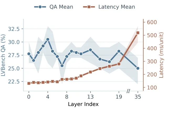
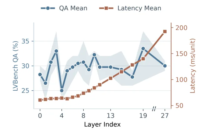
Building on this observation, ShallowStream splits the streaming pipeline into two phases (source: §4):
- Query-agnostic stream processing — encodes incoming frames with only the shallow layers and maintains a lightweight full-history index from their KV cache.
- Query-time answering — a lightweight gate decides whether history retrieval is needed, and only when it is does it concentrate full-depth computation on the retrieved evidence.
In short, the strategy is “skim shallowly in the ordinary flow, and re-examine in depth only the relevant scenes when a question arrives.” Expensive deep-layer computation is deferred until the evidence a question actually needs is pinpointed (source: §1).
Background: The Problem They Tackled
MLLM-based streaming video understanding is a core capability for real-time applications such as embodied intelligence, autonomous driving, industrial monitoring, surveillance and early warning, and wearable assistants (source: Abstract). Unlike offline long-video understanding, streaming settings require causally processing an open stream when neither future frames nor future questions are known (source: §2).
The authors explicitly point to three challenges shared by prior work (source: §1):
- Expensive Stream Processing — KV-centric methods such as ReKV, StreamMem, and InfiniPot-V prefill every frame through the full Transformer stack without knowing future questions. Even if the cache is later compressed, the computation already paid cannot be undone, and it produces deep KV cache that may never be attended to (source: §1).
- Lossy Evidence Reduction — query-agnostic compression, merging, and eviction to save memory risk discarding evidence that future retrospective queries will need. Conversely, preserving the full state makes memory balloon and forces reliance on bandwidth-limited offloading (source: §1).
- Inefficient History Use — always appending history to the context increases latency and interferes with current-scene awareness. On the other hand, approaches that trigger retrieval only when needed, such as OASIS and WeaveTime, spend one expensive answer-level reasoning pass on routing itself, and then a second reasoning pass once retrieval is activated (source: §2).
To summarize these three problems in one sentence: existing methods overlook the “model depth” dimension — this is the paper’s core diagnosis (source: Abstract).
The New Approach: ShallowStream
ShallowStream keeps a pretrained MLLM as is but redesigns where (shallow/deep layers), when (stream/query time), and what (only the selected evidence) is computed. There is no additional training at all (training-free) (source: §5).
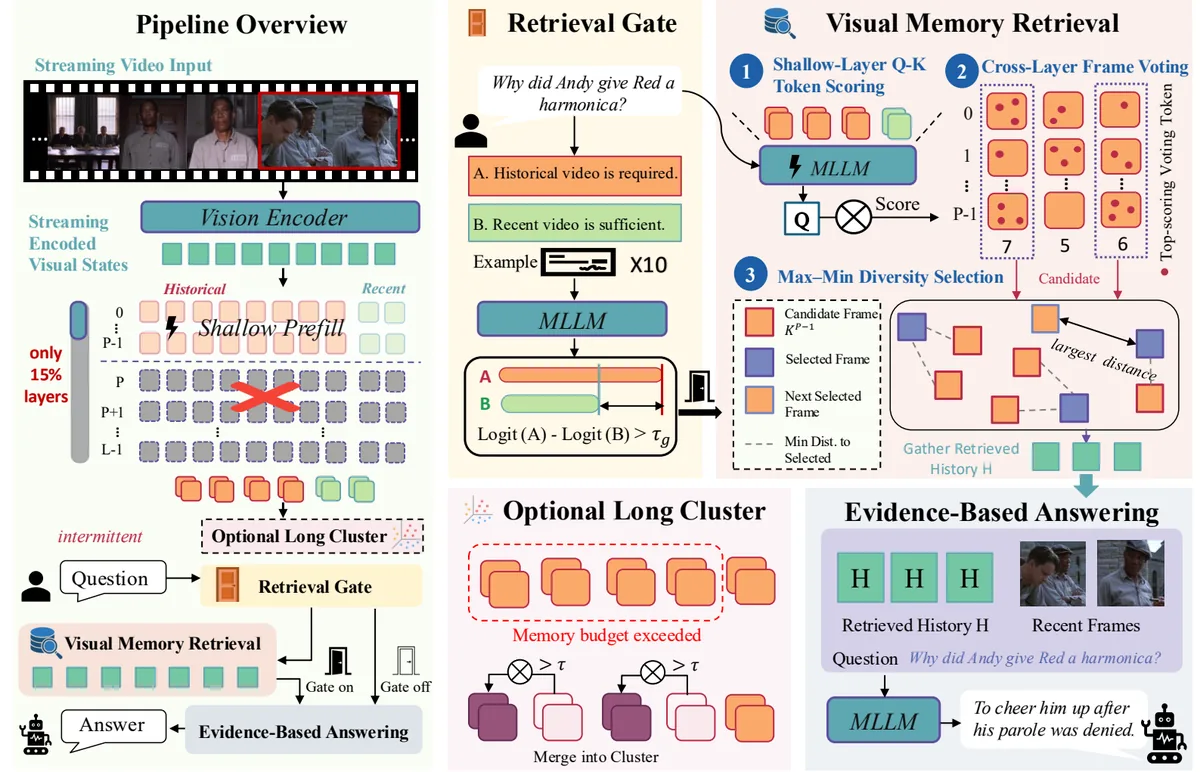
The overall pipeline is as follows (source: Fig. 3):
1) Query-Agnostic Shallow Index Construction (§4.1)
- Streaming shallow prefill — each video unit $x_t$ becomes $\bm{H}_t^0$ through the vision encoder $E_{\mathrm{v}}$, and passes through only the shallow layers $[0, P)$ to produce retrieval KV. Because the deep layers $F^P, \dots, F^{L-1}$ are skipped, per-unit computation drops from $L$ layers to $P$ layers (source: §4.1). Here the pruning boundary $P$ is 5 for Qwen3-VL-8B and 4 for LLaVA-OneVision-7B (source: Tab. Appx).
- Full-history shallow cache — the shallow KV of every observed unit is preserved: $$ \mathcal{C}_T^{\mathrm{shallow}} = \left\{ (\bm{K}_{1:T}^{i}, \bm{V}_{1:T}^{i}) \right\}_{i=0}^{P-1} $$ Cache size shrinks to roughly $P/L$ compared with preserving full depth (source: §4.1).
- Per-unit diversity descriptor — keys from the last shallow layer are averaged and $\ell_2$-normalized into a fixed-length descriptor $\bm{k}_t$ (source: Eq. 3).
- Selective long-cluster compression — when history exceeds budget $B$, older units are grouped into temporally adjacent clusters that keep fixed-size representative KV. Host-to-device transfer per cluster is fixed at one representative regardless of member count (source: §4.1).
2) Query-Time Answering (§4.2)
- Query-logit gate — the question is placed into a 10-shot routing prompt, and the logit difference of a single-token choice (A: past memory needed / B: recent scene suffices), $\ell_{\mathrm{ret}} - \ell_{\mathrm{recent}}$, is compared against a threshold $\tau_g$. Routing finishes in a single text forward, so there is no separate router training and no expensive reasoning pass (source: §4.2). The threshold is set once on a benchmark-independent calibration set and then fixed (source: §4.2, Appx).
- Token voting — when the gate activates retrieval, the last prompt token computes RoPE-aware attention scores attending to all history visual tokens at each shallow layer. The top $M=64$ tokens are drawn from each layer, and each history unit receives votes equal to the number of selected tokens belonging to it (source: §4.2).
- Max-min diversity selection — after keeping the top $4K$ candidates by vote ranking, the method starts from the farthest pair and iteratively adds the candidate whose minimum cosine distance to the selected set is largest, so the budget is not wasted on duplicate scenes. Finally $K=8$ units are chosen, and each unit gets its temporal neighbor (the immediately preceding unit) attached (source: §4.2).
- Selective re-prefill — only the input states $\bm{H}_t^0$ of the selected units are gathered and passed together with the question through all $L$ layers from scratch to generate the answer. Shallow KV is used solely to decide “what to look at in depth”; partially computed states are not carried over into generation (source: §4.2).
How It Works: A Concrete Walkthrough
Let us trace the pipeline with a very small toy example. Assume Qwen3-VL-8B ($L=28$ layers total, $P=5$, video unit = 2 frames).
Step 1 — Stream time: encode shallowly only
Video units arrive in sequence: $x_1, x_2, x_3, \dots$ Each unit passes through the vision encoder to become $\bm{H}_t^0$ and goes through only layers 0–4 to produce $(\bm{K}_t^i, \bm{V}_t^i)_{i=0}^{4}$. Layers 5–27 are never touched. Per-unit computation thus drops to about $5/28 \approx 17.9\%$ of the full cost (source: §4.1).
Meanwhile, the keys of the last shallow layer (layer 4) are averaged and normalized into a per-unit descriptor $\bm{k}_t$, stored one by one. Now memory accumulates only “shallow KV + descriptors” — far lighter than keeping full-depth KV.
Step 2 — Question arrives: the gate decides
The user asks “Where did I put the keys early in the video?” This question goes into the 10-shot routing prompt and the next-token logits are read. If $\ell_{\mathrm{ret}} - \ell_{\mathrm{recent}} \geq \tau_g$, it is classified as A (past needed) and retrieval is activated. In contrast, a question like “What color is the vehicle on screen right now?” is classified as B (recent scene suffices) and only the recent context is used (source: §4.2). This decision costs a single text forward of about 92.7 ms (source: Tab. Appx).
Step 3 — Evidence selection via token voting
Once retrieval is activated, the question tokens attend to all stored history tokens at shallow layers 0–4. In this small example, suppose there are only three candidate units. Drawing the top 64 tokens at each shallow layer and tallying the votes might give the following per-unit counts:
| Unit | $x_1$ (early scene) | $x_2$ (middle scene) | $x_3$ (recent scene) |
|---|---|---|---|
| Votes $v_t$ | 9 | 1 | 0 |
$x_1$ receives an overwhelming number of votes. Now max-min diversity selection applies. If several scenes closely resemble $x_1$, then after the first pick the method preferentially adds the scene “most different from what has already been chosen.” As a result, complementary scenes are selected instead of duplicates up to $K=8$ units (source: the qualitative case in Fig. 6 shows this effect directly).
Step 4 — Re-examine only the selected evidence in depth
Only the inputs $\bm{H}_t^0$ of the selected units are gathered and passed together with the question through all of layers 0–27. That is, rather than re-reading the whole stream in depth, only the scenes the retrieval pointed to are recomputed at full depth (source: §4.2).
The key point is this: ordinary stream processing stays cheap at $P$ layers, and the expensive $L$-layer computation is spent only on the evidence a question has pinpointed.
Performance Evaluation: Key Results
Accuracy — on par with SOTA, but far cheaper
ShallowStream matches the strongest streaming methods on both backbones (source: Tab. 1, Tab. 2).
| Benchmark | Qwen3-VL-8B + ShallowStream | LLaVA-OneVision-7B + ShallowStream |
|---|---|---|
| OVO-Bench (Avg) | 69.5 | 62.2 |
| StreamingBench (Avg) | 78.2 | 75.5 |
On OVO-Bench with Qwen3-VL-8B, it surpasses OASIS (67.7), the strongest prior baseline, recording an average of 80.9 on real-time visual perception (Real-Time) and 58.1 on retrospective tracking (Backward Tracing) (source: Tab. 1). The noteworthy benchmark is Backward Tracing: retrospective questions that can only be solved by “recalling past scenes,” it directly tests whether ShallowStream’s shallow retrieval genuinely resurrects past evidence. ShallowStream scores 58.1 on this section, higher even than OASIS (57.2) (source: Tab. 1).
Efficiency — a sharp cut to the continuous stream cost
Accuracy is maintained while costs drop substantially. The key metrics are per-frame prefill (the primary cost of stream processing) and 10-second end-to-end latency (source: Fig. 1).
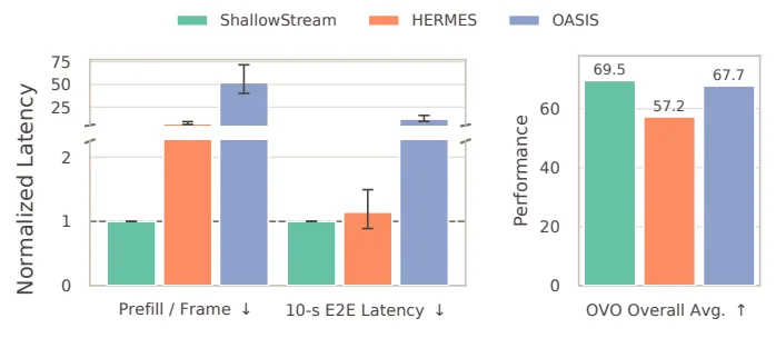
| Metric | Reduction |
|---|---|
| Per-frame prefill | up to 52.1× |
| 10s end-to-end latency | up to 11.9× |
The concrete numbers are equally clear (source: Tab. Appx):
| Measurement | Value |
|---|---|
| Stream prefill ($P=5$) | 10.72 ms/frame |
| Stream prefill ($P=19$) | 15.53 ms/frame |
| Full query (matching LC-off) | 1.759 s/query |
| Gate | 92.7 ms/query |
| Evidence selection | 106.0 ms/query |
$P=5$ keeps the best accuracy with 31.0% less per-frame prefill than $P=19$ (source: Appx). The gate and evidence selection account for only about 11% of the total per-query computation.
From a memory standpoint, enabling long-cluster compression (LC-on) keeps peak GPU memory nearly flat at about 18 GiB over the 64–1024 frame range, whereas uncompressed (LC-off) grows to 21.76 GiB. HERMES and OASIS demand more GPU memory at long prefixes (source: Fig. 4-left, §5).
From a real-time headroom standpoint, at an 80-second question interval ShallowStream spends about 2.6 seconds of total computation, while HERMES spends 6.2 seconds and OASIS spends 50.4 seconds (source: Fig. 4-right, §5). In other words, only ShallowStream operates stably below the real-time boundary.
Contribution of the Gate and Retriever (Ablation)
- The gate activates retrieval selectively, only for retrospective questions. Routing behavior differs clearly between Backward and Real-Time questions, showing that retrieval follows “historical need” rather than being indiscriminate (source: Fig. 5-left, §5).
- Token voting provides a stronger evidence-selection signal than pooled shallow Q-K or a standalone SigLIP encoder, and max-min diversity suppresses duplicate selections for further gains (source: Fig. 5-right, §5).
The qualitative cases make this effect visible too. For the question “Where is the red checkered rug?” (correct answer E), pooled Q-K repeatedly selects similar kitchen views and answers B incorrectly, whereas token voting + diversity selection selects complementary views of the whole room and gets E right (source: Fig. 6, §5).
Our Perspective: Strengths, Limitations, and Why It Matters
Strengths
- Opens a new axis: model depth. Prior efficiency work (token pruning, merging, quantization, retrieval, offloading) all touched “token count” or “cache storage,” but ShallowStream controls when full depth is executed (source: §2, §4). This is orthogonal to existing techniques, so the combination potential is high.
- No additional training at all. The gate merely reuses the logits of the pretrained model; no separate router is trained (source: §4.2). It is a drop-in method that can be attached to any offline MLLM.
- Gate calibration is benchmark-independent. Setting the threshold with synthetic questions rather than evaluation-set labels is an impressive design choice aimed at avoiding evaluation bias (source: §4.2, Appx).
Limitations
- A “Work in Progress” notice indicates the review is still at an unfinished stage (source: title footnote).
- The gate recall on the LLaVA backbone is low at 44.00% (Qwen3-VL achieves 97.00%). That is, on LLaVA, more than half of the questions that should be judged “past needed” are misrouted to “recent suffices.” Still, the precision-first design (precision 97.78%) keeps actual retrieval activation reliable (source: Tab. Appx).
- Long-cluster compression is approximate (lossy). Because only one cluster representative is consumed, member-level fine-grained evidence is not recoverable. When uncompressed fits in memory, this approximation is turned off (source: §4.1). That is, a direct evaluation of how much accuracy drops on very long streams is still missing.
- Evaluation is confined to 1 FPS sampling and fixed 16-token generation, measured on a single GPU (RTX 5090) (source: §5). Behavior at higher frame rates, longer generations, and multi-GPU scaling is unverified.
Why It Matters
Streaming video understanding is a domain where “a frame every second” is routine and “the occasional question” is the event. The first-order term of system cost should then obviously be per-frame prefill, yet prior work has consistently failed to treat it as a first-class cost (source: §1). ShallowStream elevates the empirical finding that “shallow layers suffice for retrieval” into a system design principle, establishing an operating point that cuts the continuous stream cost by more than an order of magnitude with little sacrifice in performance (source: Abstract, §6).
What’s Next?: The Road Ahead
The authors do not explicitly list future directions at length, but reasonable next steps can be read from the paper’s structure and limitations.
- Improving gate robustness — there is room to improve routing on low-recall backbones like LLaVA, or to quantitatively compare the logit-based gate with other on-demand approaches (OASIS, WeaveTime) (source: §2, Appx).
- Quantifying the compression–accuracy trade-off on very long streams — a head-to-head comparison against uncompressed is needed to see how accuracy changes as the approximation loss of long clusters accumulates (source: §4.1).
- Combining with other efficiency techniques — token pruning, quantization, and offloading are orthogonal to ShallowStream’s depth control, so verifying the gains under stacked application is a natural follow-up (source: §2).
- Scaling verification — beyond the 1 FPS / RTX 5090 / fixed 16-token setup, behavior at high frame rates, long generations, multi-GPU, and edge-device deployment needs to be checked (source: §5).
In summary, ShallowStream breaks the implicit assumption that “every frame must be read to the end,” and convincingly shows that deferred depth is a valid way to capture both performance and efficiency in streaming video understanding. Index shallowly, and answer deeply only when needed — intuitive, yet an idea no one had seriously pushed before.
Tables from the paper
Tables converted mechanically from the arXiv e-print LaTeX source. The numbers are the paper’s own and did not pass through a model.
Table 1. Main results on the OVO-Bench. Baseline results marked with $\ddagger$ are from our controlled reruns. Results marked with $\dagger$ enable long-cluster compression. Dashes indicate unreported entries.
| Model / Method | #Frames | Real-Time Visual Perception OCR | Real-Time Visual Perception ACR | Real-Time Visual Perception ATR | Real-Time Visual Perception STU | Real-Time Visual Perception FPD | Real-Time Visual Perception OJR | Real-Time Visual Perception Avg. | Backward Tracing EPM | Backward Tracing ASI | Backward Tracing HLD | Backward Tracing Avg. | Avg. |
|---|---|---|---|---|---|---|---|---|---|---|---|---|---|
| Open-source Online MLLMs | |||||||||||||
| VideoLLM-online-8B | 2 fps | 8.1 | 23.9 | 12.1 | 14.0 | 45.5 | 21.2 | 20.8 | 22.2 | 18.8 | 12.2 | 17.7 | 19.3 |
| Flash-VStream-7B | 1 fps | 25.5 | 32.1 | 29.3 | 33.7 | 29.7 | 28.8 | 29.9 | 36.4 | 33.8 | 5.9 | 25.4 | 27.6 |
| Dispider-7B | 1 fps | 57.7 | 49.5 | 62.1 | 44.9 | 61.4 | 51.6 | 54.6 | 48.5 | 55.4 | 4.3 | 36.1 | 45.3 |
| TimeChat-Online-7B | 1 fps | 75.2 | 46.8 | 70.7 | 47.8 | 69.3 | 61.4 | 61.9 | 55.9 | 59.5 | 9.7 | 41.7 | 51.8 |
| StreamForest-7B | 1 fps | 68.5 | 53.2 | 71.6 | 47.8 | 65.4 | 60.9 | 61.2 | 58.9 | 64.9 | 32.3 | 52.0 | 56.6 |
| Streamo-7B | 1 fps | 79.2 | 57.8 | 75.0 | 49.4 | 64.4 | 70.1 | 66.0 | 54.6 | 52.0 | 31.7 | 46.1 | 56.1 |
| Offline-to-Online Methods | |||||||||||||
| LLaVA-OneVision-7B | 32 | 66.4 | 53.2 | 71.6 | 51.1 | 72.3 | 59.2 | 62.3 | 53.9 | 52.7 | 18.8 | 41.8 | 52.1 |
| + ReKV | 0.5 fps | 52.4 | 54.1 | 69.8 | 43.3 | 67.3 | 57.1 | 57.3 | 57.6 | 56.1 | 18.8 | 44.2 | 50.8 |
| + HERMES$^{\ddagger}$ | 0.5 fps | 71.1 | 61.5 | 74.1 | 52.3 | 72.3 | 66.3 | 66.3 | 62.0 | 60.8 | 26.9 | 49.9 | 58.1 |
| + WeaveTime | 1 fps | 72.5 | 69.7 | 74.1 | 53.4 | 75.2 | 67.9 | 68.8 | – | – | – | – | – |
| + CausalMem | 0.5 fps | 71.8 | 61.5 | 76.7 | 48.9 | 76.2 | 66.8 | 65.7 | – | – | – | – | – |
| + SimpleStream$^{\ddagger}$ | 4 | 77.2 | 71.6 | 75.9 | 52.3 | 77.2 | 71.7 | 71.0 | 53.2 | 52.0 | 43.6 | 49.6 | 60.3 |
| + ShallowStream (Ours) | 1 fps | 87.3 | 73.4 | 77.6 | 62.9 | 74.3 | 77.2 | 75.4 | 50.2 | 50.7 | 46.2 | 49.0 | 62.2 |
| + ShallowStream (Ours)$^{\dagger}$ | 1 fps | 87.3 | 73.4 | 77.6 | 63.5 | 74.3 | 77.2 | 75.5 | 50.5 | 50.7 | 46.2 | 49.1 | 62.3 |
| Qwen3-VL-8B | 64 | 76.5 | 58.7 | 75.0 | 59.0 | 68.3 | 59.2 | 66.1 | 53.2 | 66.9 | 9.7 | 43.3 | 54.7 |
| + HERMES$^{\ddagger}$ | 2 fps | 85.2 | 64.2 | 73.3 | 55.6 | 70.3 | 65.8 | 69.1 | 50.5 | 65.5 | 19.9 | 45.3 | 57.2 |
| + OASIS | – | 92.0 | 80.7 | 81.0 | 67.4 | 67.3 | 79.9 | 78.1 | 62.0 | 60.1 | 47.3 | 57.2 | 67.7 |
| + SimpleStream$^{\ddagger}$ | 4 | 92.0 | 81.7 | 81.9 | 69.7 | 75.3 | 81.0 | 80.2 | 53.2 | 60.1 | 44.1 | 52.5 | 66.4 |
| + ShallowStream (Ours) | 1 fps | 92.0 | 83.5 | 82.8 | 71.9 | 75.3 | 79.9 | 80.9 | 52.5 | 72.3 | 49.5 | 58.1 | 69.5 |
| + ShallowStream (Ours)$^{\dagger}$ | 1 fps | 92.0 | 83.5 | 82.8 | 71.9 | 76.2 | 79.9 | 81.0 | 51.2 | 71.0 | 50.0 | 57.4 | 69.2 |
Table 2. Main results on the Real-Time Visual Understanding subset of StreamingBench. Baseline results marked with $\ddagger$ are from our controlled reruns. Results marked with $\dagger$ enable long-cluster compression. Dashes indicate unreported results.
| Model / Method | #Frames | Real-Time Visual Understanding OP | Real-Time Visual Understanding CR | Real-Time Visual Understanding CS | Real-Time Visual Understanding ATP | Real-Time Visual Understanding EU | Real-Time Visual Understanding TR | Real-Time Visual Understanding PR | Real-Time Visual Understanding SU | Real-Time Visual Understanding ACP | Real-Time Visual Understanding CT | Avg. |
|---|---|---|---|---|---|---|---|---|---|---|---|---|
| Open-source Online MLLMs | ||||||||||||
| Flash-VStream-7B | – | 25.9 | 43.6 | 24.9 | 23.9 | 27.3 | 13.1 | 18.5 | 25.2 | 23.9 | 48.7 | 23.2 |
| VideoLLM-online-8B | 2 fps | 39.1 | 40.1 | 34.5 | 31.1 | 46.0 | 32.4 | 31.5 | 34.2 | 42.5 | 27.9 | 36.0 |
| Dispider-7B | 1 fps | 74.9 | 75.5 | 74.1 | 73.1 | 74.4 | 59.9 | 76.1 | 62.9 | 62.2 | 45.8 | 67.6 |
| TimeChat-Online-7B | 1 fps | 80.2 | 82.0 | 79.5 | 83.3 | 76.1 | 78.5 | 78.7 | 64.6 | 69.6 | 58.0 | 75.4 |
| StreamForest-7B | 1 fps | 83.1 | 82.8 | 82.7 | 84.3 | 77.5 | 78.2 | 76.9 | 69.1 | 75.6 | 54.4 | 77.3 |
| Offline-to-Online Methods | ||||||||||||
| LLaVA-OneVision-7B | 32 | 77.7 | 76.6 | 77.6 | 81.9 | 71.7 | 71.7 | 66.7 | 65.5 | 65.7 | 44.0 | 71.0 |
| + ReKV | 0.5 fps | 74.4 | 78.9 | 78.6 | 77.1 | 68.3 | 67.9 | 67.6 | 62.6 | 64.3 | 44.6 | 69.2 |
| + HERMES$^{\ddagger}$ | 0.5 fps | 78.2 | 79.7 | 86.8 | 81.5 | 69.2 | 73.2 | 75.0 | 64.2 | 68.6 | 45.6 | 73.2 |
| + StreamKV | 1 fps | 74.7 | 78.1 | 87.7 | 79.4 | 70.8 | 67.6 | 70.4 | 64.6 | 64.0 | 45.1 | 71.0 |
| + WeaveTime | 1 fps | 71.5 | 81.3 | 86.8 | 78.6 | 75.2 | 73.2 | 72.2 | 69.1 | 68.8 | 44.7 | 72.1 |
| + SimpleStream$^{\ddagger}$ | 4 | 80.4 | 71.9 | 85.2 | 85.5 | 76.1 | 73.8 | 69.4 | 65.5 | 71.1 | 37.3 | 73.5 |
| + LiveVLM | 0.5 fps | 79.8 | 79.7 | 84.9 | 80.7 | 67.1 | 70.1 | 74.1 | 66.3 | 68.0 | 42.5 | 71.3 |
| + CausalMem | 0.5 fps | 82.6 | 79.7 | 83.2 | 83.2 | 69.6 | 78.4 | 75.0 | 67.3 | 70.9 | 39.4 | 74.3 |
| + ShallowStream (Ours) | 1 fps | 82.8 | 67.2 | 83.9 | 90.8 | 71.7 | 81.9 | 64.8 | 70.7 | 74.8 | 35.2 | 75.5 |
| + ShallowStream (Ours)$^{\dagger}$ | 1 fps | 82.8 | 67.2 | 83.9 | 90.8 | 72.3 | 81.9 | 64.8 | 70.7 | 74.8 | 35.2 | 75.6 |
| Qwen3-VL-8B | 64 | 80.4 | 75.0 | 83.0 | 83.5 | 74.2 | 84.4 | 77.8 | 63.8 | 69.7 | 57.0 | 75.9 |
| + SimpleStream$^{\ddagger}$ | 4 | 79.3 | 72.7 | 89.9 | 84.8 | 73.6 | 79.1 | 83.3 | 71.1 | 76.8 | 39.4 | 76.5 |
| + HERMES$^{\ddagger}$ | 2 fps | 79.0 | 77.3 | 81.4 | 84.2 | 73.6 | 77.9 | 87.0 | 70.7 | 72.5 | 61.1 | 76.6 |
| + ShallowStream (Ours) | 1 fps | 79.3 | 71.9 | 89.9 | 85.8 | 77.4 | 79.1 | 88.9 | 71.5 | 77.3 | 52.9 | 78.2 |
| + ShallowStream (Ours)$^{\dagger}$ | 1 fps | 79.3 | 71.9 | 90.2 | 85.5 | 77.4 | 79.1 | 88.9 | 71.5 | 77.3 | 49.7 | 78.0 |
Table 3. Main implementation settings for the two evaluated backbones.
| Setting | Qwen3-VL-8B | LLaVA-OneVision-7B |
|---|---|---|
| Backbone and Stream Processing | ||
| Pruning boundary $P$ | 5 | 4 |
| Sampling rate, OVO / StreamingBench | 1 / 1 FPS | 1 / 1 FPS |
| Video unit | 2 frames | 1 frame |
| Stream prefill window | 64 units, 128 frames | 128 units, 128 frames |
| Query Routing | ||
| Gate prompt | ten shot | ten shot |
| Gate calibration set | 200 shared query-only examples | |
| Gate threshold $\tau_g$ | 11.0 | 0.875 |
| Evidence Selection and Generation | ||
| Query representation | last prompt token | |
| Visual candidates per shallow layer | 64 tokens | |
| Vote-ranked candidate pool | 32 historical units | |
| Selected historical evidence | 8 units with max-min diversity | |
| Temporal expansion | one preceding unit per selected unit | |
| Recent context, retrieval / recent-only | 6 / 2 units | |
| Maximum new tokens | 16 |
Table 4. Cost summary under the final calibrated Gate and token-vote retriever. Stream-time prefill is averaged over the same five long videos; query components use the matched full-history LC-off setting.
| Measurement | Setting or component | Cost |
|---|---|---|
| Stream-time prefill | $P=1$ | $9.47$ ms/frame |
| $P=5$ | $10.72$ ms/frame | |
| $P=19$ | $15.53$ ms/frame | |
| Query-time computation | Full query | $1.759$ s/query |
| Gate | $92.7$ ms/query | |
| Evidence selection | $106.0$ ms/query |
Table 5. Query-logit Gate calibration on the benchmark-independent query-only set.
| Backbone | $\tau_g$ | Precision | 95% lower bound | Recall |
|---|---|---|---|---|
| Qwen3-VL-8B | 11.0 | 96.04% | 91.47% | 97.00% |
| LLaVA-OneVision-7B | 0.875 | 97.78% | 90.63% | 44.00% |
Figures in this post are taken from the original arXiv:2609.02780 (CC BY 4.0). Only size and format were changed.
Comments