Introduction
In settings where the batch size is close to 1, such as conversational services, the latency of a mixture-of-experts language model comes mostly from reading the routed expert weights from GPU memory. Most of the intermediate dimensions inside an expert contribute little to a token, so choosing which channels to read first can substantially reduce the amount read. This paper shows that two objectives that existing channel selectors try to meet through calibration data are in fact not achieved, and presents a selector built from model weights alone, without calibration.
Background: Channels and Retention Rules
In an MoE layer, the router sends a token to a few experts. An expert is a gated MLP. Each intermediate dimension of this expert is called a channel. Channel $j$ owns the $j$-th row of the gate matrix $G_e$ and the up matrix $V_e$, and the $j$-th column of the down matrix $D_e$.
Given an input $x$, channel $j$ computes the following.
- Gate activation: $\phi(g_j^\top x)$
- up output: $(v_j^\top x)$
- Channel activation: $a_j = \phi(g_j^\top x)(v_j^\top x)$
The full routed output is the sum of the $a_j d_j$ produced by each channel, scaled by the expert’s router weight.
For illustration, consider Qwen3-Thinking (the actual structure in §2). A single token goes to 8 experts, and each expert has 768 channels. So at each layer the selector must choose what to read among $8 \times 768 = 6144$ candidate channels. Once it decides to compute channel $j$, it reads row $j$ of gate/up and column $j$ of down, computes $a_j d_j$ exactly, and adds it to the output. Discarded channels are not read at all (as shown later, the reader fills them in approximately).
The central fork in a channel selector is the retention rule. Even with the same scores, the way of deciding which channels to keep changes the amount read and the accuracy.
| Rule | Input | State | Change | Output |
|---|---|---|---|---|
| Threshold $\tau$ | Same score for tokens A and B | Channels with score $\ge \tau$ pass | A keeps 6, B keeps 2 | Amount read varies per token |
| top-k ($k=4$) | Same score | Top 4 scores pass | Both A and B keep 4 | Amount read is fixed per token |
A threshold is intended to give each token as much as it needs, but the actual amount read moves with the input. top-k fixes the amount in advance, but keeps $k$ channels regardless of what the token actually needs.
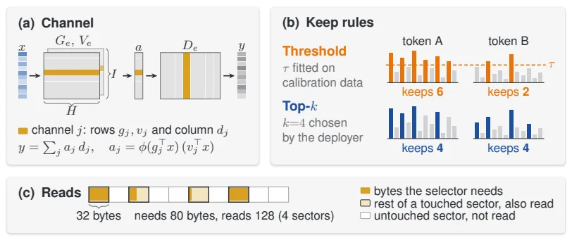
Consider Fig. 2 of the original. (a) draws the structure in which channel $j$ owns row $j$ of gate/up and column $j$ of down. (b) shows the difference that, at the same score, a threshold changes the retention count per token while top-k fixes it. (c) shows how cost is computed. Modern NVIDIA GPUs fetch memory in 32-byte sectors, so when the needed bytes are scattered, every touched sector is charged in full.
| Small example (c) | Value |
|---|---|
| Bytes the selector actually needs | 80 bytes |
| Sectors those bytes occupy | 4 (scattered) |
| Sectors the hardware touches | All 4 |
| Read charged | $4 \times 32 = 128$ bytes |
The paper calls this cost reads. It is the bytes read per token measured as a percentage of the full model’s routed expert reads. The accounting was also checked against a profiler to confirm it matches actual hardware transfers. For batch-1 Qwen3-Thinking, cold-cache DRAM reads are 18.3%, close to the accounted 17.8% (Appendix C).
Read savings are not compute (FLOPs) savings. They are the gain from reading fewer weights in a memory-bandwidth-bound setting.
Calibration Fails Both Promises
A channel selector uses a calibrated threshold for two reasons: to know the amount read in advance, and to improve accuracy by giving tokens the channels they need at that amount. The authors break each of these in turn with experiments.
A Threshold Does Not Fix the Amount Read
The threshold $\tau$ is fixed, but the number of channels crossing it varies with the input.
Consider an experiment that computes channel scores exactly as their actual contribution to the output and calibrates $\tau$ so that about 12% is retained on UltraChat. On separate conversational data not used for calibration, the average retention count matched the target. Yet even on the same conversational data, the middle 90% of Qwen3-Thinking tokens retain only 9.0–16.2%, a wide spread, and on benchmark answers (GPQA-Diamond, IFEval, MMLU-Pro) the scores become smaller, dropping the median to 10.0%.
The retention count decreases as answers get longer. Around 6,000 answer tokens, Qwen3-Thinking retains only 71% of the calibrated count, Gemma 4 92%, and Qwen3.5 88%.
In actual deployment it is simpler. Across all 72 benchmark runs we performed, selectors using a calibrated threshold read less than the target. Prox was calibrated to 18% but actually reads 12.9% on average and as little as 9.9%. The reader’s threshold version also meets the target on calibration data but reads 0.4–5.8%p less on benchmarks (§4.1).
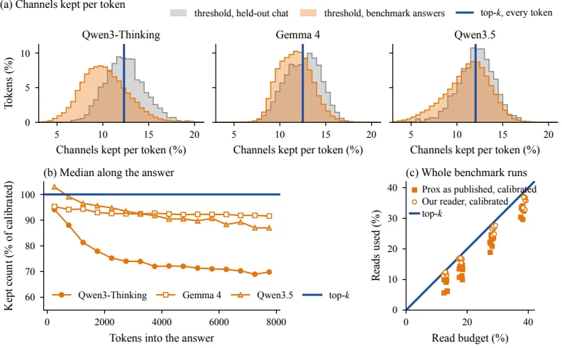
Let us read Fig. 4 of the original. (a) is the distribution of the channel retention ratio per token. The orange threshold curve meets the target on the chat data used for calibration, but on benchmark answers the median drops to 10%. The thick line is top-k, which keeps the same ratio for every token. (b) plots, as the median over 500-token windows, what percentage of the calibrated value the retention count is at each answer length. (c) plots actual amount read against the budget on the horizontal axis. Every point lies below the diagonal, that is, short of the target.
We also checked why it decreases. The retention count follows the answer written so far rather than how much the token needs. At the threshold Prox calibrated to 13%, if the 256-token window at position 6,000 of a Qwen3-Thinking GPQA-Diamond answer is detached from its preceding context and placed immediately after the question, the same tokens retain 57% more channels. Nor do harder tokens receive more channels. The correlation between retention count and the full model’s next-token loss is only −0.29 to +0.14 (§4.1, Appendix E).
Calibration Gives No Consistent Accuracy Gain over top-k
To compare the two retention rules, the scores must be fixed. The authors ran each selector twice with the same channel scores: once with a calibrated threshold and once with top-k. At budgets of 13% and 18%, with generation tasks on 4 MoE models and a likelihood task on OLMoE, and with 3 kinds of scores (Prox, TEAL, and Prox scaled at the output level), they produced 43 comparisons in total.
| Same scores, two retention rules compared (§4.2) | Result |
|---|---|
| Ties (within 2 standard errors) | 30 |
| top-k ahead | 10 |
| Threshold ahead | 3, with a margin of at most 2.8 points |
That is, in 40 of 43, top-k matches or wins. Here a tie means no difference was detected, not equivalence. Grouped by model as well, no model prefers the threshold at the calibration budget (Appendix Table 14).
Even in a check favorable to the threshold, which reruns the top-k version at the amount the threshold version actually read, top-k matches or wins in 37 of 41 (Appendix F, Fig. 8).
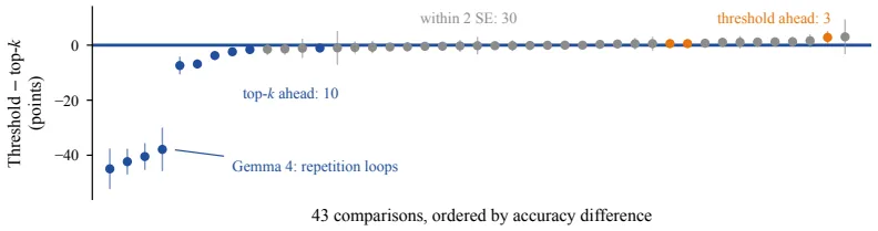
In Fig. 5 of the original, each point is one comparison. The vertical axis is the threshold version’s accuracy minus the top-k version’s, so below 0 (blue) is a top-k win. Gray is a tie, the 10 blue points are top-k wins (four of them from Gemma 4 at 38–45 points), and only 3 orange points are threshold wins (at most 2.8 points). This figure is based on the calibration budget; the version rerun at actual reads is in Appendix Fig. 8.
Long Reasoning Can Collapse under a Calibrated Threshold
The four largest gaps in Fig. 5 all come from Gemma 4. At the 13% budget, top-k with Prox (and its output-scaled variant) beat the threshold version by 38–45 points.
Gemma 4 with the calibrated threshold repeats sentences and reaches the 32,768-token limit. This is not because it reads less.
| Condition (Gemma 4, GPQA-Diamond) | Prox threshold (calibrated to 18%) | Prox top-k |
|---|---|---|
| Actual reads | 13.3% | 13.5% |
| Accuracy | 11.7 | 56.3 |
| Reaching the limit out of 792 answers | 674 | 145 |
The cause was also narrowed down. Changing only Prox’s channel threshold to top-k makes the collapse disappear. Changing only the input threshold does not. Neither flooring the channel minimum retention at 4% nor recalibrating on Gemma 4’s own reasoning prevents the collapse (§4.3, Appendix D.1, F.2).
The authors conjecture that this collapse acts like a cliff. Once a sparse model starts repeating, it is hard to stop on its own, and when the error that sparsification adds per token exceeds some model-specific level, accuracy falls sharply rather than gradually. This explanation is a hypothesis, not a proof (§4.3).
A Reader Built from Weights Alone
When top-k is the retention rule, performance depends on two things: how well channels are ranked before reading, and how discarded channels are handled. The observation that changing the scores moves KL divergence far more than changing the retention rule set the design direction of the reader (§5).
The reader is built once from model weights before deployment. It has no values calibrated to the target model. Three settings—128-coordinate rotation blocks, an 80-coordinate partial scan, and rank-32 recovery—are fixed once on OLMoE development data and reused for all models. For each token and layer, the reader runs three stages. It screens all candidate channels, computes the top $k$ exactly, and recovers the rest.
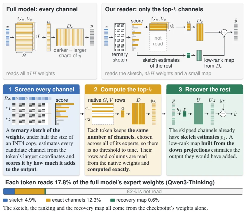
Consider Fig. 6 of the original. The top contrasts the full model, which reads all channels of the routed experts, with the reader, which reads a ternary sketch, the real weights of the retained $k$ channels, and a recovery map. The middle shows the behavior of the three stages. The bottom breaks down the 17.8% reads on Qwen3-Thinking. The sketch accounts for 4.9%, the exactly computed channels for 12.3%, and the recovery map for 0.6%, while the remaining roughly 82% is not read at all.
Stage 1: Screen with a Ternary Sketch
Weights and hidden states have outliers that make low-bit codes inaccurate. So the gate row $g_j$ and up row $v_j$ are rotated in 128-coordinate blocks by a random Hadamard transform $R$, spreading large values evenly within the block. $R$ is orthogonal, so the rotation does not change the activation ($g_j^\top x = (Rg_j)^\top(Rx)$).
The rotated blocks are stored as follows.
| Stored item | Value | Role |
|---|---|---|
| Ternary code | $\{-1,0,1\}$ | Stand-in for the weights |
| FP16 scale | 1 per block | Restores the code to its actual magnitude |
| $\rho_b$ | Mean-squared quantization error of the block | Used to rank channels by the error remaining after recovery at high budgets |
A block shrinks from 256 bytes in BF16 to about 30 bytes, so the sketch adds about 7% to resident memory. At decode time, $x$ is rotated once and multiplied with the sketch to obtain $\hat g_j \approx g_j^\top x$, $\hat v_j \approx v_j^\top x$ (§5.1).
At low budgets such as 12.8% and 17.8%, reading the entire sketch alone accounts for 44–61% of all reads (for OLMoE). So a partial scan is used. From each block, only the ternary codes of the 80 coordinates with the largest $|Rx|$ are read. This increases the number of exactly computed channels by 20–50% at the same budget (§5.1).
Stage 2: Compute the Top k Exactly with Output-Level Scores
The magnitude that channel $j$ adds to the output is $w_j\,\lVert d_j\rVert\,|a_j|$. Here $w_j$ is the router weight, and $\lVert d_j\rVert$ is the norm of the down column, computed once at load time. Replacing the activation $a_j$ with the sketch estimate gives the score
$$s_j = w_j\,\lVert d_j\rVert\,\bigl|\phi(\hat g_j)\,\hat v_j\bigr|$$(Equation 1). Because the score is at the output level, channels from different experts can be compared directly. So the top $k$ are chosen across all experts the token passes through. One expert may receive many channels and another none at all (§5.2).
The $k$ channels remaining after screening have their real weights read to compute $a_j$ exactly. To read the down weights contiguously, the down projection is transposed once at load time so that prefill and decode use the same layout.
Stage 3: Recover Discarded Channels with a rank-32 Map
The contribution of a single discarded channel is small, but thousands per layer add up to something not negligible. The screening stage has already computed an activation estimate $p_j = \phi(\hat g_j)\hat v_j$ for every discarded channel, so it is reused without reading gate/up again. The remaining problem is the down column $d_j$ of each discarded channel.
Instead of reading full-width columns, all down columns of the layer are stacked to obtain the top 32 left singular vectors $U \in \mathbb{R}^{H \times 32}$, and the coefficient $b_j = U^\top d_j$ of each channel is stored. The final output is
$$\hat y = \sum_{j \in K} w_j d_j a_j \;+\; U\sum_{j \in S} w_j b_j p_j.$$The first term is the exact contribution of the retained $K$ channels. The second term adds the estimated contribution of the discarded $S$ channels via the rank-32 map (Equation 2). The map adds about 0.5% to resident memory and 0.5–0.8%p to reads (§5.3).
Accuracy and Speed
Accuracy
Accuracy was evaluated on 9 pairs of three post-trained models (Qwen3-Thinking, Gemma 4, Qwen3.5) and three benchmarks (GPQA-Diamond, IFEval, MMLU-Pro). The full model processes the prompt, and the selector runs for each subsequent decoding token. Accuracy is reported as a percentage of the full model’s accuracy. The table below reconstructs only the rows needed for the roughly 18% budget from Table 1. For calibrated selectors, both the target and the actual reads are listed.
| Selector (roughly 18% budget) | Target | Actual reads | Mean | Worst |
|---|---|---|---|---|
| Our reader | – | 17.8 | 98.1 | 95.0 |
| Prox score, top-k | – | 18.5 | 96.1 | 90.4 |
| Prox as published, calibrated | 18 | 12.9 | 68.5 | 12.1 |
| WINA as published, top-k | – | 20 | 28.4 | 1.1 |
| TEAL as published, calibrated | 20 | 12.6 | 9.9 | 0.0 |
The reader is the most accurate at both low budgets. At 17.8% it averages 98.1% and 95.0% on the worst pair. At 12.8% it still averages 94.5% and 86.9% on the worst pair, better than the worst pair of any other selector.
The notable place is Prox. It was calibrated to 18% but actually reads 12.9%, similar to the reader’s 12.8%, yet its mean accuracy is only 68.5%. Most of the gap comes from Gemma 4’s repetition loop. On the two Qwen models, Prox matches the reader at similar reads. top-k does not rescue a weak score either. WINA with top-k reaches only 28.4% even at 20% reads (§6.1).
Speed
Speed must be viewed separately as kernel performance and full-system performance. The Triton kernel was compared at 17.8% reads, on a single RTX PRO 6000 Blackwell GPU, against the fastest configuration of unmodified vLLM.
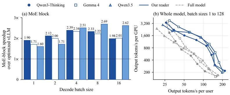
Fig. 7 (a) of the original is decode speedup of the MoE block alone. At batch 1 it is 1.90x for Qwen3-Thinking, 1.71x for Gemma 4, and 1.60x for Qwen3.5. At batch 4 it is 2.39/2.34/2.51x, and the maximum is 2.69x for Qwen3.5 at batch 8.
(b) is full-model performance. Further right means faster per user, and higher means more output per GPU. Because attention is unchanged the gain is small: 1.15–1.36x at batch 1, peaking at 1.75/1.74/1.88x at batch 8–16, and converging to 1.00–1.24x at batch 128 (Table 20). On long contexts of 8k–32k tokens it is 1.08–1.54x.
The reason the gain at batch 1 is smaller than the read savings is fixed cost. On Qwen3-Thinking, even though the MoE block accounts for only 18.3% of full-model memory traffic, the block is only 1.90x faster rather than 5x. Fixed costs such as kernel launch do not shrink with read savings. As the batch grows, these fixed costs are shared, so block speedup increases up to batch 4–8. But as the batch grows further, the union of channels selected by the tokens grows again, increasing the amount that must be read and reducing the gain (§6.2, Appendix J).
Limitations and When to Apply It
The authors acknowledge five limitations (§7).
- The kernel converts only part of the read savings into speed. It is tuned for one budget (17.8%) and one GPU type.
- Selecting channels for the whole batch at once so that the gain carries to large batches is future work.
- The number of coordinates in the partial scan (80 of 128) was set on OLMoE and confirmed only on Gemma 4.
- The reader changes only the routed experts during decoding. The sketch and recovery map add about 7% and 0.5% to a BF16 checkpoint, and their share is larger in quantized checkpoints.
- The tested models are at most 35B parameters.
There are also two patterns the authors conjecture hold more broadly. These are conjectures, not verified results (§7). One is that short likelihood evaluations hide failures in long generation, and the other is that low KL divergence does not imply high accuracy.
From a reviewer’s perspective, the remaining condition is this. The conclusion is limited to ’the case of using a calibrated threshold on the channels of frozen MoE experts.’ The authors themselves state that thresholds may be valid elsewhere, such as in sparse attention or learned routers (§3). The cliff explanation is also a hypothesis, not a proof.
The operational sweet spot is the decode stage when serving a post-trained MoE model at small batch while the prompt is processed by the full model. Conditions not yet verified are very large batches beyond 128, other GPU types, quantized checkpoints (confirmed only on OLMoE), and the prefill stage.
Tables from the paper
Tables converted mechanically from the arXiv e-print LaTeX source. The numbers are the paper’s own and did not pass through a model.
Table 1. Our reader is the most accurate tested selector at the two lowest budgets. Mean and worst accuracy over nine model-benchmark pairs, as a percentage of the full model’s accuracy. Selectors with calibrated thresholds list the budget they were calibrated for (Target) and the reads they used (Realized); WINA as published uses top-$k$ and meets its budget to the precision shown.
| Selector | About 13% of reads Target | About 13% of reads Realized | About 13% of reads Mean | About 13% of reads Worst | About 18% of reads Target | About 18% of reads Realized | About 18% of reads Mean | About 18% of reads Worst |
|---|---|---|---|---|---|---|---|---|
| Our reader | – | 12.8 | 94.5 | 86.9 | – | 17.8 | 98.1 | 95.0 |
| Prox score, top-$k$ | – | 13.5 | 87.0 | 61.1 | – | 18.5 | 96.1 | 90.4 |
| Prox as published, calibrated | 13 | 8.5 | 51.5 | 0.0 | 18 | 12.9 | 68.5 | 12.1 |
| WINA as published, top-$k$ | – | 15 | 2.4 | 0.0 | – | 20 | 28.4 | 1.1 |
| WINA score, calibrated | 15 | 7.8 | 0.2 | 0.0 | 20 | 11.2 | 5.0 | 0.0 |
| TEAL as published, calibrated | 15 | 8.9 | 0.2 | 0.0 | 20 | 12.6 | 9.9 | 0.0 |
Table 2. Prior keep-rule comparisons reach opposite conclusions, focus mostly on short tasks on dense models, and none runs top-$k$ at the reads a threshold actually uses. Unlike most prior comparisons, ours holds the channel score fixed (Same score), tests long chain-of-thought reasoning on MoE models (Regime), and runs top-$k$ both at the target budget and at realized reads (Matched).
| Study | Regime | Models | Same score | Matched | Ahead |
|---|---|---|---|---|---|
| La RoSA | dense, PPL | LLaMA2-7B | yes | target | top-$k$ (PPL) |
| Batch-wise pruning | dense, CoT | 2 distilled 7–8B | yes | target | top-$k$ (batch 4) |
| Sparsing Law | dense, short tasks | 0.1B, 0.8B | no | target | threshold |
| Prox | dense, short tasks | Qwen3-8B, 14B | yes | target | threshold (+1.8) |
| TopK-Guided | dense, short tasks | Llama-2/3, 7–8B | no | target | hybrid; top-$k$ vs.\ $\tau$ mixed |
| Sparser-MoE | MoE, short tasks | OLMoE | unclear | target | top-$k$ ($<$1 pt) |
| This paper (\S) | MoE, short + CoT | 4 MoE models | yes | both | tie; top-$k$ on Gemma 4 |
Table 3. Evaluated MoE models and the resident memory our reader adds. Each row gives the number of routed experts and how many each token uses, the channels per expert and the hidden width, the number of MoE layers, any module that always runs in full, and the resident memory of our reader’s ternary sketch and recovery map as a percentage of the BF16 checkpoint. OLMoE’s sketch size is computed analytically.
| Model | Routed experts Total | Routed experts Active | Width Expert | Width Hidden | MoE layers | Always full | Added memory (%) Sketch | Added memory (%) Recovery |
|---|---|---|---|---|---|---|---|---|
| Qwen3-Thinking | 128 | 8 | 768 | 2048 | 48 | – | 7.6 | 0.50 |
| Gemma 4 | 128 | 8 | 704 | 2816 | 30 | dense MLP | 7.0 | 0.35 |
| Qwen3.5 | 256 | 8 | 512 | 2048 | 40 | shared expert | 7.0 | 0.47 |
| OLMoE | 64 | 8 | 1024 | 2048 | 16 | – | 7.3 | 0.50 |
Table 4. Evaluation protocol on the post-trained models. Each model runs in thinking mode with its model card’s sampling parameters and random seed 20260923. GPQA-Diamond reports accuracy over four samples per question, IFEval reports prompt-level strict accuracy, and MMLU-Pro reports accuracy on a fixed 1,000-question subset.
| Model | Benchmark | Items | Samples | Sampling Temperature | Sampling Top-$p$ | Sampling Top-$k$ | Sampling Max tokens |
|---|---|---|---|---|---|---|---|
| Qwen3-Thinking | GPQA-D | 198 | 4 | 0.6 | 0.95 | 20 | 32,768 |
| IFEval | 541 | 1 | 0.6 | 0.95 | 20 | 32,768 | |
| MMLU-Pro | 1,000 | 1 | 0.6 | 0.95 | 20 | 32,768 | |
| Gemma 4 | GPQA-D | 198 | 4 | 1.0 | 0.95 | 64 | 32,768 |
| IFEval | 541 | 1 | 1.0 | 0.95 | 64 | 32,768 | |
| MMLU-Pro | 1,000 | 1 | 1.0 | 0.95 | 64 | 32,768 | |
| Qwen3.5$^{\dagger}$ | GPQA-D | 198 | 4 | 1.0 | 0.95 | 20 | 81,920 |
| IFEval | 541 | 1 | 1.0 | 0.95 | 20 | 32,768 | |
| MMLU-Pro | 1,000 | 1 | 1.0 | 0.95 | 20 | 32,768 | |
| $^{\dagger}$Presence penalty 1.5. |
Table 5. Most of our reader’s reads go to exact channels, and the sketch takes most of the rest. Routed-expert reads per token at batch one, as a percentage of the full model, by component at the four main budgets. At the two smallest budgets, the partial screen reads part of the ternary sketch.
| Model | Sketch read | Routed-expert reads (%) Sketch | Routed-expert reads (%) Exact channels | Routed-expert reads (%) Recovery | Routed-expert reads (%) Metadata | Routed-expert reads (%) Total |
|---|---|---|---|---|---|---|
| Qwen3-Thinking | partial | 4.86 | 7.29 | 0.66 | 0.04 | 12.85 |
| partial | 4.86 | 12.30 | 0.63 | 0.04 | 17.83 | |
| full | 7.99 | 20.00 | 0.59 | 0.10 | 28.68 | |
| full | 7.99 | 30.00 | 0.54 | 0.10 | 38.62 | |
| Gemma 4 | partial | 4.78 | 7.49 | 0.54 | 0.03 | 12.84 |
| partial | 4.78 | 12.50 | 0.52 | 0.03 | 17.83 | |
| full | 7.86 | 19.99 | 0.49 | 0.08 | 28.42 | |
| full | 7.86 | 30.01 | 0.45 | 0.07 | 38.40 | |
| Qwen3.5 | partial | 5.08 | 6.98 | 0.74 | 0.04 | 12.84 |
| partial | 5.08 | 12.04 | 0.72 | 0.04 | 17.87 | |
| full | 8.33 | 20.00 | 0.68 | 0.11 | 29.11 | |
| full | 8.33 | 30.00 | 0.62 | 0.10 | 39.06 |
Table 6. Our reader reads part of the sketch at the two smallest budgets and all of it above. Each column is one budget. It gives the share of candidate channels computed exactly across each token’s routed experts and the resulting total reads, which include the ternary sketch, exact channels, recovery map, and metadata, averaged over the three post-trained models and three benchmarks.
| Sketch read | partial | partial | full | full | full | full |
|---|---|---|---|---|---|---|
| Channels computed exactly (%) | 7.0–7.5 | 12.0–12.5 | 20 | 30 | 50 | 70 |
| Reads (% of full model) | 12.8 | 17.8 | 28.7 | 38.7 | 58.6 | 78.5 |
Table 7. At batch one, the profiler measures 18.3% of the full model’s DRAM reads, close to the 17.8% we count. Measured DRAM reads per MoE layer on Qwen3-Thinking in MB, averaged over 12 layers, without the router, with a cold cache.
| Batch size | 1 | 4 | 8 |
|---|---|---|---|
| Full model | 75.6 | 229.1 | 359.3 |
| Our reader | 13.9 | 49.9 | 92.3 |
| Share | 18.3% | 21.8% | 25.7% |
Table 8. Every calibrated threshold reads less than the budget it was calibrated for. Each row is one selector at one calibrated budget. The columns give the lowest, mean, and highest realized routed-expert reads (%) over the nine model-benchmark pairs.
| Method | Calibrated for (%) | Realized reads (%) Min | Realized reads (%) Mean | Realized reads (%) Max |
|---|---|---|---|---|
| CATS | 53.3 | 51.1 | 52.1 | 53.0 |
| 66.7 | 63.8 | 65.1 | 66.0 | |
| Our reader, calibrated | 12.8 | 11.2 | 11.8 | 12.4 |
| 17.8 | 15.2 | 16.5 | 17.1 | |
| 28.7 | 24.5 | 26.5 | 27.7 | |
| 38.7 | 32.9 | 35.8 | 37.2 | |
| Prox as published, calibrated | 13.0 | 5.6 | 8.5 | 10.1 |
| 18.0 | 9.9 | 12.9 | 14.7 | |
| 28.0 | 18.9 | 22.5 | 24.6 | |
| 38.0 | 29.6 | 32.6 | 34.1 | |
| 58.0 | 47.3 | 49.8 | 51.0 | |
| 78.0 | 67.1 | 70.0 | 71.4 | |
| TEAL as published, calibrated | 15.0 | 6.4 | 8.9 | 11.0 |
| 20.0 | 9.8 | 12.6 | 15.3 | |
| 30.0 | 19.9 | 22.6 | 24.9 | |
| 40.0 | 32.6 | 35.0 | 36.2 | |
| 50.0 | 43.7 | 46.2 | 47.4 | |
| 60.0 | 54.7 | 56.9 | 58.0 | |
| WINA score, calibrated | 15.0 | 5.4 | 7.8 | 9.6 |
| 20.0 | 8.2 | 11.2 | 13.9 | |
| 30.0 | 17.2 | 20.7 | 23.5 | |
| 40.0 | 32.0 | 34.3 | 35.8 | |
| 50.0 | 43.5 | 46.1 | 47.7 | |
| 60.0 | 54.8 | 57.1 | 58.2 |
Figures in this post are taken from the original arXiv:2610.37386 (CC BY 4.0). Only size and format were changed.
Comments