Paper Recent language models keep increasing the amount of information packed into a single vocabulary entry. Per-layer embeddings (PLE), first introduced in Gemma 3n, carried over to Gemma 4: instead of a single input-layer vector per vocabulary item, each decoder layer has a different learned vector. This post examines OPTIC, which shrinks this table by about 100× while retaining most of the original performance, starting from the problem setting and proceeding through a small example, the method, results, and limitations.
OPTIC’s core ideas are two. One is to store a single code per token and have each layer unfold that code with its own decoder; the other is to fit the codes and decoders not by “how faithfully the stored vectors are reconstructed” but by “how much difference appears in the output path the model actually uses.”
Why PLE is a problem
A typical input embedding turns one token into one vector. For the token "cat", it simply retrieves the single vector that the token points to in the vocabulary dictionary. PLE adds a layer axis on top of this. Even for the same token, the vector used at layer 1 differs from the vector used at layer 42, and each layer retrieves its vector from its own stage’s residual connection. The residual connection is the pathway that adds a term to the hidden state as it passes through each layer.
Storage grows immediately. E4B has a vocabulary of 262,144, 42 decoder layers using PLE, and a vector width of 256 dimensions, so storing a separate vector for each token-layer pair results in 11 million token-layer vectors (§1, §2.2). In bfloat16 that is about 5.64GB (§2.2). In the same checkpoint, PLE accounts for 35.2% of parameters (abstract). In the smaller E2B it is 45.8% (§1).
Illustrative example: let’s see what a single token actually stores and does (E4B).
| Step | State |
|---|---|
| Input | One token ID (e.g. "cat") |
| Stored state | 42 256-dim vectors, one per layer = 42×256 = 10,752 numbers, 21,504 bytes in bfloat16 |
| What happens at a layer | That layer’s vector is multiplied elementwise by the gate and projected to the hidden width by the output projection matrix |
| Output | The PLE residual added to the hidden state |
Compressing this table by about 100× leaves just over 5 bytes per vector (§1). Existing quantization methods spend those few bytes on “a code per vector.” With 11 million vectors each having its own code, the codes become far too short and reconstruction quality drops sharply.
How OPTIC stores and reconstructs
The problem is clear. 5 bytes is not enough to properly hold a single vector. The PLE table has two directions, the token axis and the layer axis, and OPTIC shares both directions at once (§2.2).
- Token direction: instead of each token storing its 42 vectors separately, each token stores one code.
- Layer direction: all tokens in a layer share a single affine decoder (matrix multiply plus addition). The size of this decoder is independent of vocabulary size.
Concretely, token t stores M indices. Each index points to a 4-dimensional codeword in its own codebook, and concatenating the M of them yields a latent vector z_t that summarizes the token. Then layer ℓ unfolds z_t into a 256-dim row with its own affine decoder.
In the ~100× setting for E4B, M=161 and 256 codewords (K=256) are used. A single token needs to store only 161 indices, i.e. 161 bytes, reducing 21,504 bytes of 42 vectors to 161 bytes (§2.2). In exchange, the codebook (about 330KB) is shared fully, and the decoder weights (~13.8MB) and biases of the 42 layers are shared by all tokens in the respective layer. Total is 56.4MB, 99.94× versus the original 5.64GB (§2.2, Table 16).
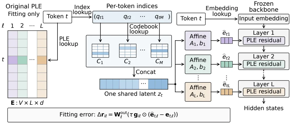
Reading the figure above as a state transition: the input is a single ID for token t. The stored state is the M indices placed in vocabulary row t (e.g., 161 bytes). Each index q_{tm} selects one row (highlighted cell) of its own codebook C_m, and concatenating the 161 selected codewords computes the latent vector z_t (length 644). At this point the layer does not intervene yet. Then layer ℓ applies its own affine weight A_ℓ and bias b_ℓ to compute the 256-dim row ê_{tℓ}, and that row leads to the PLE residual of layer ℓ. Cells of the same color indicate the same layer, and the dashed ellipsis indicates omitted layers and codebooks. Importantly, the original PLE is used only in the “fitting step” and not for actual storage and reconstruction (original Figure 1).
The key point is that the cost of storing indices is now proportional only to vocabulary size V and not to V × L. Conventional row-wise quantization must store an index set per vector, which multiplies by the number of layers, whereas OPTIC removes this layer factor (§2.2, Equation 3).
Why fit on the “output path”
Sharing storage alone is not the end. PLE vectors are not used on their own; at each layer they pass through the gate and output projection and are added to the hidden state. Specifically, the PLE row is multiplied elementwise by a gate derived from the layer’s hidden state, then projected to the hidden width by the output projection matrix W_out (§2.3).
Therefore, what matters more directly to model quality is not how similar the reconstructed vector is “in coordinates” to the original, but how much difference remains after passing through the gate and output projection. OPTIC fits the codes and decoders to minimize the error in this projected output rather than in the stored coordinates (§2.3, Equation 4–5).
$$ \Delta r_{i\ell}(\theta) = W^{\mathrm{out}}_\ell \bigl( \tau\, g_{i\ell} \odot (\hat e_{\theta, t_i \ell} - e_{t_i \ell}) \bigr) $$Here g_{iℓ} is the gate at calibration position i and layer ℓ, τ is a fixed PLE scale, and ⊙ is elementwise multiplication. Gates from the training records are collected from the pre-compression model and used fixed. Gates for synthetic records are filled with 1 (§3.2). The objective is the mean of this projected output error ‖Δr‖² over positions and layers (§2.3, Equation 5).
The fitting procedure alternates two kinds of updates (§2.4, Algorithm 1). One updates the codebooks and decoders continuously (with AdamW) while fixing the codes; the other reassigns each token’s index to the codeword with the smallest error while fixing the codebooks. Reassignment covers all tokens in the vocabulary. To handle rare tokens that do not appear often in natural-language calibration, it uses a per-layer averaged gate metric G_ℓ as a surrogate objective (§2.4, Equation 6–7). Initialization concatenates per-token vectors, subtracts the vocabulary mean, and builds the latent vectors and decoders via PCA scaled by the output-path weights, then starts with an OPQ-style assignment that splits coordinates into codebook groups and runs K-means within each group.
Results: quality preserved, memory reduced
Quality first. The paper reports the geometric mean of “retention relative to the original” across 7 tasks (PIQA, GSM8K, GPQA Diamond, AIME 2026, MMLU-Redux, IFBench, InfographicVQA). Each task’s retention is capped at 100%, so over-performance on one task cannot mask losses on another. If any single task scores 0, the geometric mean becomes 0 (§3.3, Equation 8).
Question: at ~100× compression, how well do existing quantization methods and OPTIC hold up? Below are the E4B results (Table 1).
| Method | BF16 retention | W4A16 retention |
|---|---|---|
| PQ | 66.3% | 82.4% |
| AQLM Euclidean beam encoder | 46.7% | 82.8% |
| Output-path weighted PCA-PQ | 93.3% | 88.3% |
| OPTIC | 97.8% | 96.9% |
| Frequency-tiered OPTIC | 95.7% | 95.1% |
On BF16 E4B, OPTIC leads the strongest existing method (PQ) by 31.5 percentage points, and on W4A16 it leads the strongest method (AQLM) by 14.0 percentage points (§4.1). On E2B, OPTIC retains 89.1% on BF16 and 91.5% on W4A16, while the frequency-tiered variant is highest at 90.0% and 93.0% (§4.1, Table 1). The frequency-tiered variant gives more code groups to frequent tokens, uses learned shared codewords per group for the remaining tokens, and preserves exactly the PLE rows of special tokens in bfloat16 (§2.5, Appendix A.3).
Looking at actual task scores shows where the difference comes from. On BF16 E4B, GSM8K is 92.8% for OPTIC versus 92.9% original and 73.5% for PQ. IFBench is 41.7% for OPTIC versus 44.0% original and 16.0% for PQ, and InfographicVQA is 67.5% for OPTIC versus 69.7% original and 38.4% for PQ (§4.1, Table 12). The drop for existing methods is especially large in mathematical reasoning, instruction following, and visual question answering. Bootstrap 95% confidence intervals also separate. On BF16 E4B, OPTIC is 95.5–99.0% and PQ is 60.6–70.5%. On W4A16 E4B, OPTIC is 93.9–97.8% and AQLM is 76.8–87.1% (Table 2). These intervals reflect benchmark sampling uncertainty.
OPTIC holds up even at higher compression rates. The curve below plots retention (y-axis) against compression rate (x-axis, log scale).
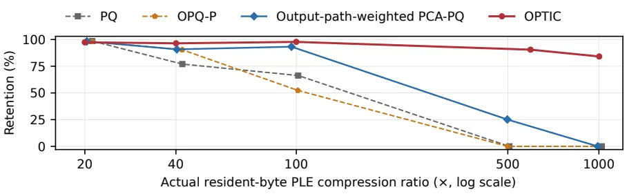
Dashed lines are existing methods (PQ, OPQ-P), solid lines are the authors’ method. OPTIC retains 97.8% at ~100×, and still holds 90.5% and 84.1% at 594× and 1002×. W4A16 E4B at the same points is 87.7% and 81.8% (§4.2, Table 16). In contrast, output-path weighted PCA-PQ, which improves only row-wise, is good at 93.3% near 100× but falls to 25.1% near 500× and reaches 0 near 1000× (§4.2). The fewer bytes left per vector, the larger the benefit of sharing codes at the token level.
Kernel speed and system performance are measured separately
Beyond quality, how memory and time behave in actual serving is a separate measurement. The authors compared original PLE and ~100× compressed PLE in vLLM on a single RTX 4090 under identical settings (fixed 1GiB KV cache) (§6).
Memory drops substantially from a system perspective. For BF16 E4B, process GPU memory falls from 18.57GB to 13.05GB, a 29.7% reduction, and for W4A16 it falls from 12.95GB to 7.37GB, a 43.1% reduction (Table 7). This is because the PLE resident on the GPU shrinks from 5.64GB to 56.4MB.
Time must be read from both a kernel and a system perspective. In single-lookup measurements where the table is in host memory, dense lookup is faster for a single token (compressed lookup is 0.6×), but from 32 tokens compressed lookup becomes faster, reaching 12.1× at 8192 (Table 11). In terms of total serving time, compressed PLE is only up to 0.40% slower on BF16 and up to 0.69% slower on W4A16 (Table 9). Compressed lookup must perform extra multiplications to unfold codes with the decoder, so under the same cache budget the conclusion is “memory drops a lot, time stays about the same.”
However, situations where memory is the real bottleneck are different. Under the same GPU budget, there are cases where dense PLE either fails to start because it does not fit in the KV cache or processes requests sequentially, while compressed PLE cuts completion time by up to 2.1× (§B.3, Table 10). In other words, the goal is not saving serving time per se; the gain appears when memory becomes latency.
Why this works
Start with the analysis showing that layer averaging alone is insufficient. Replacing each vector wholesale with its layer’s vocabulary mean drops GSM8K from 92.9% to 43.5%, GPQA from 56.9% to 23.0%, and AIME to 0, even though the mean vector accounts for only 8.1% of the table’s total squared norm (§5.1, Appendix E.3). In other words, the information that differs per token is the core of performance.
So is that per-token variation concentrated in low dimensions? The next figure answers this question.
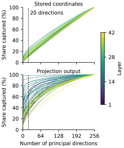
The top panel shows stored coordinates and the bottom panel shows coordinates after output projection; each curve (layer) shows how many principal components explain the per-token variation (x-axis: number of principal components, y-axis: cumulative explained ratio). In stored coordinates, 212–227 directions are needed to explain 90%. After output projection, this drops to 1–205 per layer (median 158) (§5.1, Figure 3). This gap is the basis for OPTIC’s choice to “fit on the output path.” After the gate and projection, important variation is concentrated substantially toward lower dimensions, a signal that a low latent width can be tolerated to some degree.
There are also experiments that isolate and validate the two designs. One is the effect of code sharing. If each token-layer vector gets an independent latent code and the same fitting procedure is applied, E4B BF16 retention drops from 97.8% to 79.3% at nearly the same storage budget (Table 3). The caveat that this difference mixes the effect of sharing itself with the effect of reallocating bytes between codes and decoders is revisited in the limitations section. Decoder freedom also matters. If only the decoder is refit by least squares with indices, codebooks, and biases fixed while limiting rank to 20 per layer, retention drops from 95.09% to 70.55% (§5.2, Table 4).
The other is the effect of output-path fitting. With codes and initialization fixed and only the objective changed, the context-dependent output-path objective gives 1.98 percentage points higher retention on average than Euclidean error and 0.31 percentage points higher than the diagonal approximation (§5.3, Table 5). Also, continuous updates produce most of the gain (63.60% with initialization only, 94.67% with continuous updates), and index reassignment adds 0.65–1.14 percentage points on top (§5.3, Table 6).
Limitations and applicability
To decide whether to use OPTIC in practice, one must separate the limitations the authors state from other conditions.
Start with the limitations the authors state explicitly. Evaluation is limited to Gemma 4 E2B/E4B, and the main comparison uses a single fixed fitting seed, so confidence intervals reflect only benchmark sampling uncertainty (Limitations). The six baselines are reconstructions of the original papers’ methods adapted to PLE, and cannot be read directly against results from their original settings (Limitations). The code-sharing ablation also mixes in the effect of reallocating bytes between codes and decoders, so it does not measure only the “pure sharing effect” (Limitations). Calibration adds synthetic records (gate = 1) covering the full vocabulary to 786,432 natural-language positions (§3.2), so tokens that rarely appear in natural language are fitted with synthetic records alone. The output-path loss is also an approximation that measures error only at each layer’s projected output with gates fixed (Limitations).
From a reviewer’s perspective, three things are worth noting. First, the method is specialized for embeddings with a “token×layer” structure like PLE, so the benefit does not carry over directly to ordinary single input embeddings, which lack the layer axis for code sharing. Second, retention is a geometric mean over 7 tasks, and any single task scoring 0 makes the whole thing 0, so if a low-sample task collapses the metric swings sharply. One should check individual scores to see whether a particular task collapses under extreme compression (1000×), but the paper does not report per-task scores for extreme compression (Tables 12 and 13 contain only the 100× condition; those numbers are not reported in the original). Third, the serving gains above depend on a memory-bottleneck condition, so there is less to expect in environments without it.
In conclusion, OPTIC is promising for settings where “the embedding table makes up a large part of the model and GPU memory is constrained,” especially when serving PLE-family models with many concurrent requests. It can also be combined with W4A16 weight-only quantization. The perspective of fitting where the model actually consumes the vectors rather than where they are stored shows that embedding capacity and compressed representation can be designed together from the start (Conclusion).
Tables from the paper
Tables converted mechanically from the arXiv e-print LaTeX source. The numbers are the paper’s own and did not pass through a model.
Table 1. PLE compression on the original BF16 and official W4A16 releases at the nominal $100\times$ tier. Cells report compression ratio $R$ / seven-task retention (%) relative to the matched uncompressed PLE. A zero denotes at least one zero task score. Bold marks the highest retention in each column.
| Method | Original BF16 E2B $R$ / Retention | Original BF16 E4B $R$ / Retention | Official W4A16 E2B $R$ / Retention | Official W4A16 E4B $R$ / Retention |
|---|---|---|---|---|
| Baselines | ||||
| PQ | 101.24/22.9 | 101.43/66.3 | 101.24/0.0 | 101.43/82.4 |
| RVQ | 100.96/0.0 | 98.64/37.6 | 100.96/29.3 | 101.20/82.0 |
| OPQ-P | 100.92/0.0 | 101.16/52.4 | 100.92/0.0 | 101.16/57.9 |
| AQ | 100.96/0.0 | 101.20/45.6 | 100.96/0.0 | 101.20/62.8 |
| AQLM Euclidean beam encoder | 100.96/20.7 | 101.20/46.7 | 100.96/32.0 | 101.20/82.8 |
| INT8 randomized low-rank SVD | 100.13/0.0 | 99.76/37.7 | 100.13/0.0 | 100.24/51.1 |
| Our methods | ||||
| Output-path-weighted PCA-PQ | 96.14/32.2 | 96.36/93.3 | 96.14/44.5 | 96.36/88.3 |
| OPTIC | 99.86/89.1 | 99.94/97.8 | 99.86/91.5 | 99.94/96.9 |
| Frequency-tiered OPTIC | 100.48/90.0 | 100.00/95.7 | 100.48/93.0 | 100.00/95.1 |
Table 2. Paired-bootstrap confidence intervals for the four primary nominal-$100\times$ comparisons. Retention is reported in percent.
| Setting | Our method | Retention (95% interval) | Strongest baseline | Retention (95% interval) |
|---|---|---|---|---|
| E2B, BF16 | OPTIC | 89.1 [85.8, 91.8] | PQ | 22.9 [0.0, 28.8] |
| E4B, BF16 | OPTIC | 97.8 [95.5, 99.0] | PQ | 66.3 [60.6, 70.5] |
| E2B, W4A16 | OPTIC | 91.5 [89.3, 93.3] | AQLM Euclidean beam encoder | 32.0 [0.0, 38.9] |
| E4B, W4A16 | OPTIC | 96.9 [93.9, 97.8] | AQLM Euclidean beam encoder | 82.8 [76.8, 87.1] |
Table 3. Seven-task retention (%) near $100\times$ PLE compression with fit seed 0, relative to the uncompressed checkpoints of Tables and . Independent latent codes use the main method’s fitting recipe and calibration data, with 0.8–0.9% fewer resident bytes. OPTIC values are the main results of Table . Output-path-fitted additive codes keep their standard initializer.
| Representation | E2B BF16 | E4B BF16 | E2B W4A16 | E4B W4A16 |
|---|---|---|---|---|
| Independent latent codes | 28.5 | 79.3 | 53.7 | 86.8 |
| Additive codes | 42.1 | 90.0 | 83.5 | 94.4 |
| OPTIC | 89.1 | 97.8 | 91.5 | 96.9 |
Table 4. Decoder refits on the three E4B BF16 fits of Table , which use a common Euclidean initialization, near $100\times$. Values are means and sample standard deviations over fit seeds 0, 1 and 2. Refits keep each fit’s indices, codebooks and biases, constrain rank before float16 storage, and share the uncompressed reference of Table .
| Decoder refit with fixed codes | Retention (%) |
|---|---|
| Rank unlimited | $95.09\pm0.48$ |
| Fitted rank at most 20 per layer | $70.55\pm1.18$ |
Table 5. Fixed-code fitting on E4B BF16 near $100\times$, with the common Euclidean initialization and 5,000 continuous updates. Each loss is divided by its value for an all-zero reconstruction. Values are means and sample standard deviations over three fits.
| Fixed-code objective | Retention (%) |
|---|---|
| Euclidean | $92.76\pm1.16$ |
| Diagonal output path | $94.44\pm0.94$ |
| Context-dependent output path | $94.74\pm0.59$ |
Table 6. Optimization on E4B BF16 near $100\times$. Values are means and sample standard deviations over three fits. The last two rows use 5,000 continuous updates, and the final row adds 18 reassignment sweeps.
| Optimization recipe | Retention (%) |
|---|---|
| Initialization only | $63.60\pm3.68$ |
| Continuous updates only | $94.67\pm0.53$ |
| Continuous updates + reassignment | $95.49\pm0.40$ |
Table 7. Post-initialization process GPU memory for E4B on an RTX 4090 with a fixed 1 GiB key-value cache, averaged over two engine initializations. Resident PLE storage falls from 5.64 GB to 56.4 MB.
| Backbone | Dense (GB) | Compact (GB) | Saved (%) |
|---|---|---|---|
| BF16 | 18.57 | 13.05 | 29.7 |
| W4A16 | 12.95 | 7.37 | 43.1 |
Table 8. Model releases used for fitting and evaluation. The final column gives a 12-character revision prefix.
| Scale | Role | Hugging Face model | Version |
|---|---|---|---|
| E2B | Evaluated BF16 | google/gemma-4-E2B-it | b446025c61ec |
| E4B | Evaluated BF16 | google/gemma-4-E4B-it | ee0ef6023621 |
| E2B | PLE fit for W4A16 | google/gemma-4-E2B-it-qat-q4_0-unquantized | 6befbaca7398 |
| E4B | PLE fit for W4A16 | google/gemma-4-E4B-it-qat-q4_0-unquantized | 476025a01dbf |
| E2B | Evaluated W4A16 | google/gemma-4-E2B-it-qat-w4a16-ct | 971342c08f60 |
| E4B | Evaluated W4A16 | google/gemma-4-E4B-it-qat-w4a16-ct | 6cd26aaa2357 |
Figures in this post are taken from the original arXiv:2610.31309 (CC BY 4.0). Only size and format were changed.
Comments