The sequential bottleneck of sampling one token at a time
Large language models can compute an entire sentence in parallel during training, but when generating text they must know the preceding token before they can choose the next one. No matter how fast the GPU is, this order cannot be skipped in one pass, so generation latency grows. This post covers Lafa (Large flow language model), which attacks this bottleneck with block-level flow.
Lafa revives an already-trained autoregressive model. A single computation produces candidate tokens for an entire block, and autoregressive prediction verifies and commits them from the front. As a result, it achieves up to 2.54× the throughput of the existing autoregressive baseline at the same quality level. The exact conditions and numbers are revisited below.
Why flow, and why split into blocks
The existing parallel generation method, discrete diffusion, erases tokens with [MASK] and then restores them. Sampling multiple positions independently in one step severs the relationships between positions, which can degrade quality.
Flow differs: it does not erase tokens. It mixes Gaussian noise into token embedding vectors, then integrates the continuous path from noise back to clean embeddings to produce tokens. Because it moves in continuous space, the acceleration and control techniques developed for image and video generation carry over directly. However, existing flow language models were demonstrated only on small-scale, simple tasks; one scaling attempt reported training inefficiency; and how to scale to billions of parameters is not yet established (§1, §2).
Lafa splits flow into blocks. Instead of generating the whole sentence at once, it conditions on the previously committed text (the prefix) and generates token blocks of size $B$ one at a time, chaining blocks causally. The sentence probability is factorized as a product over blocks.
$$p(y\mid c)=\prod_{r} p\bigl(y^{rB+1:(r+1)B}\mid c,\,y^{\le rB}\bigr)$$Splitting into blocks yields two benefits. First, the prefix key-value (KV) cache—the attention intermediates from previous token computations—can be reused for each block. Second, parallel generation can be confined to within a block (§2.1). Handling tokens on embeddings reduces the dimensionality of a single token from the vocabulary size $|V|$ to the embedding dimension $d$, which also makes training and scaling easier.
Asynchronous flow within a block
If every position in a block escaped noise at the same rate, the left-to-right directionality of text being read would disappear. Lafa gives each position $i$ its own progress clock $\tau^i(t)$. The clocks of earlier positions run faster, so earlier tokens are revealed first. The path from noise $x_0$ to the clean embedding $x_1$ is as follows.
$$I_t^i=(1-\tau^i(t))\,x_0^i+\tau^i(t)\,x_1^i$$$\tau$ is not fixed. It is learned from data so that training passes slowly through regions with high loss. This concentrates training samples and inference steps around difficult noise levels. The learned schedule generally advances earlier positions first (in Fig. learned_time, the horizontal axis is reference time $t\in[0,1]$, the vertical axis is the per-position $\tau^i(t)$, and the curves correspond to block positions 1, 4, 7, …, 16); this left→right bias is not manually imposed but emerges from training (§2.1).
Illustrative example. Suppose the three embeddings of the prefix “the weather today is” are already committed, and with block size $B=3$ we must produce “sunny/cloudy/.”
| Step | Input | Retained state | Changing state | Output / discarded values |
|---|---|---|---|---|
| Start | 3 prefix embeddings, 3 noise vectors | prefix KV cache | — | — |
| Step $k$ | reference time $t_k$, current state $\hat x_{t_k}$ | prefix KV cache | earlier positions’ $\tau$ grow first and $\hat x$ approaches the embeddings | intermediate noise $\hat x_{t_k}$ |
| End | after $K$ Euler steps | prefix KV cache | tokens are committed from the final $\hat x$ | “sunny/cloudy/.” |
The KV of the committed tokens is appended and we move to the next block. This example is for intuition only and is unrelated to the measurements below.
Designing flow to be learned from an autoregressive model
The key is not to train a flow model from scratch but to retrofit an already-trained autoregressive model into a block denoiser. The denoiser is a function that, given a noisy block, predicts the clean-token probability at each position. The problem is that this retrofit must not damage autoregressive prediction or the prefix cache. The paper solves this with three designs (§2.2).
First, tokenwise time conditioning. The prefix receives time 1 (no noise), and each position in the block receives its own time $\tau^i(t)$. This value is injected via adaptive layer normalization (adaLN)—a mechanism that re-normalizes a layer’s output based on its input. Initializing adaLN as the identity function means time conditioning initially leaves the existing computation untouched and is learned gradually.
Second, block bidirectional attention. Tokens within a block can see each other, so less-refined later tokens can help earlier ones. The prefix is still viewed only causally, as before. As a result, the prefix’s keys and values do not depend on block state and can be reused across denoising steps.
Third, fixed embedding norm. If embeddings are updated freely, their L2 norm grows relative to the noise scale, creating a shortcut that makes denoising easier. The pretrained norm is fixed and only the direction is learned.
The training loss sums three terms: autoregressive cross-entropy on the prefix, denoising cross-entropy on block tokens, and squared error between predicted and actual embeddings (Equation 6). Keeping the autoregressive loss also improves flow accuracy. Thanks to this joint training, autoregressive ability is preserved—or even improved—while learning flow. This is consistent with the existing observation that multi-token prediction improves next-token prediction (§2.2, §3.2).
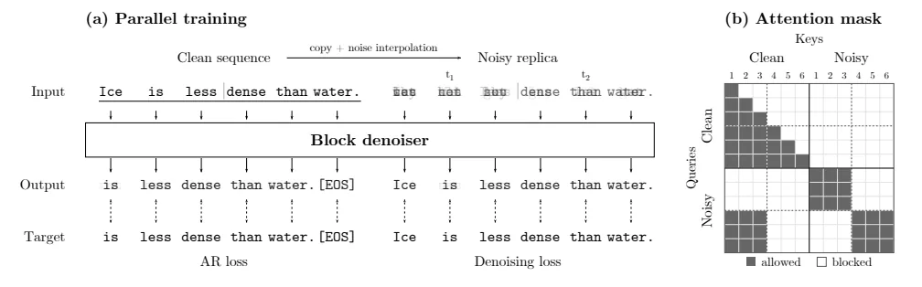
The figure above (original Figure training) shows the state transitions of parallel training. The upper clean sequence produces autoregressive predictions with causal attention, while the lower copy is split into blocks of size 3, where each block sees only the preceding clean tokens and produces denoising predictions bidirectionally within the block. A single forward pass yields both the autoregressive loss and the denoising losses of all blocks, without recomputing overlapping prefixes.
Design effects confirmed by ablation
At 0.5B, block 4, and 32 Euler steps, each design was reverted one at a time and average accuracy was compared (Table design-ablations).
| Changed item | Comparison condition | Average accuracy |
|---|---|---|
| Attention | Fully causal | 32.7% |
| Block bidirectional | 38.0% | |
| Time schedule | Synchronous (all positions share the same $t$) | 36.2% |
| Asynchronous tokenwise | 38.0% | |
| Embedding | Fully frozen | 34.4% |
| Unrestricted updates | 36.9% | |
| Fixed norm | 38.0% | |
| Loss | Denoising cross-entropy only | 33.6% |
| Squared error only | 29.7% | |
| Both terms | 35.8% | |
| Both terms + autoregressive | 38.0% |
The original design wins on all four axes: attention, time, embedding, and loss. In particular, adding the autoregressive loss actually raises flow accuracy, so AR preservation and flow generation do not hurt each other.
Reducing the number of steps with flow map distillation
Flow decoding is expensive because it must call the denoiser many times per block. To reduce this, Lafa uses flow map distillation. A student model learns a function $\hat X_{s,t}$ that moves the state directly from time $s$ to $t$, replacing several Euler steps with a single jump. Predictions on the diagonal ($s=t$) are matched to the teacher, while off-diagonal predictions ($s\lt t$) are matched to the composition of two short jumps in a semigroup fashion. The student maintains the prefix cache and can generate in as few as 1 step ($\hat X_{0,1}$) (§2.2).
Draft and verify at once: self-speculative decoding
Reaching AR-level quality with flow decoding requires many steps. Lafa discards the expensive multi-step process and by default draws a block draft with 1-step flow, then verifies it with the autoregressive predictor (§2.3).
The draft comes from a single denoiser evaluation starting from noise. Each position of the draft is compared against the autoregressive prediction from the front, and only the longest matching prefix is committed; the rest is discarded. If even the first token differs, it is replaced with the autoregressive token. The final output is exactly the same as the model’s greedy autoregressive output. Flow is used only to increase speed, and the quality bar equals greedy autoregression.
A naive implementation needs a separate verification forward and a next-draft forward, which costs extra. The paper eliminates this with fused decoding: verification of the previous draft and drafting of the next block are mixed into a single forward pass.
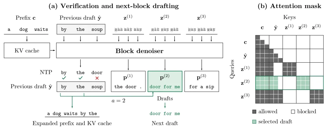
The figure above (original Figure fused_decoding) shows how one stage proceeds at block size 3. The horizontal direction is sequence position, and the vertical blocks are the input fragments fed into each forward.
| Stage | Input | Retained | Changed / rejected | Output |
|---|---|---|---|---|
| End of previous stage | prefix KV, draft $\hat y$ | prefix KV | — | — |
| Fused forward | clean draft $\hat y$ + $B$ candidate noise blocks | prefix KV | each candidate assumes “$j$ preceding items accepted” | verification logits, $B$ candidate drafts |
| Verification | verification logits vs autoregressive prediction | accepted prefix KV | drafts and candidates after the mismatch are discarded | accepted length $a$, next draft |
| Next stage | extended prefix | updated KV cache | — | repeat |
The clean draft is appended like a prefix to produce verification logits via causal attention, and at the same time candidate noise blocks corresponding to “the case where $j$ preceding draft items are accepted” are appended and processed together. From the verification result, the candidate block with the actually accepted length is chosen as the next draft, eliminating a separate re-drafting forward.
Because this method performs both drafting and verification with a single trained model, it is called self-speculative. No separate small draft model or additional parameters are needed. Alternatively, confidence decoding—accepting only prefixes whose token probability exceeds a threshold instead of using autoregressive verification—is possible, but lowering the threshold trades accuracy for speed, so the paper keeps self-speculative as the default (§3.3, Appendix confidence_results).
Results: maintaining quality while increasing speed
The models use Qwen2.5 0.5B·7B Instruct and Qwen3 8B Base as initialization and are trained for only 5–15 epochs (9–27B tokens) on Dolci-Instruct-SFT data. This is at least 18× fewer than the up to 500B tokens reported by comparable-scale diffusion models (Dream, LLaDA, Efficient-DLM) (§3, Table training-hyperparameters). The benchmarks are six covering instruction following, reasoning, and coding: IFEval, BBH, MMLU-Pro, GPQA, GSM8K, and HumanEval.
Learning flow does not hurt autoregression
Comparing average single-token decoding accuracy across the six benchmarks (Table ntp_main), Lafa beats the AR SFT built with the same initialization, data, and training budget at every scale. At 8B it approaches Efficient-DLM’s 63.5% while using at least 18× fewer training tokens. The process of learning flow actually improved autoregressive prediction (Table 1, §3.2).
| Scale | AR SFT | Lafa | Difference |
|---|---|---|---|
| 0.5B | 28.7% | 31.6% | +2.9%p |
| 7B | 58.4% | 60.9% | +2.5%p |
| 8B | 56.8% | 63.1% | +6.3%p |
Parallelism: how far does accuracy hold as TPF rises
TPF (tokens per forward) is the number of tokens committed per forward pass. For AR it is 1 by definition. Since self-speculative output equals greedy autoregression, TPF comparisons are parallelism comparisons at the same AR quality.
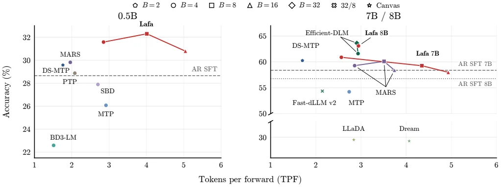
In the figure above (original Figure selfspec_frontier), the horizontal axis is TPF and the vertical axis is average accuracy over the six benchmarks. At 7B, block 4 reaches TPF 2.6 and 60.9% accuracy, beating DeepSeek-MTP on both accuracy and TPF, while block 16 reaches 58.0% at TPF 4.9, close to AR SFT’s 58.4% while nearly doubling parallelism. Across all scales, AR-level accuracy is maintained in the roughly 2.5–5 TPF range (Table selfspec_lafa_sixbench).
Wall-clock time: throughput measured in TPS
TPF shows only parallelism, not actual time. Because the cost of a forward pass differs by method, tokens per second (TPS) was measured on a single H100 GPU at batch 1.
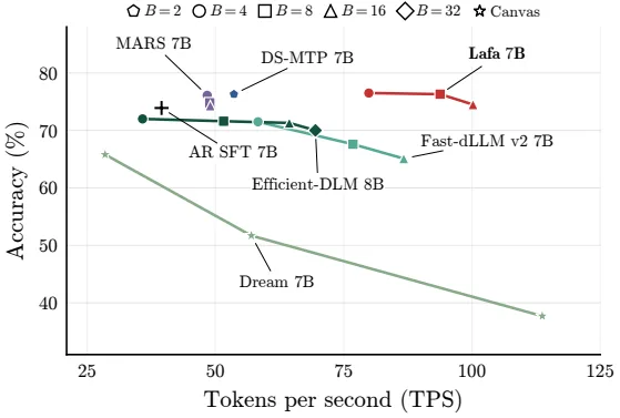
In the figure above (original Figure throughput), the horizontal axis is TPS and the vertical axis is average accuracy over IFEval, GSM8K, and HumanEval. Lafa 7B with block 16 reaches 100.2 TPS, 2.54× the throughput of AR SFT’s 39.5 TPS at similar average accuracy (74.5% vs 73.9%). With block 4 it is about 2× faster at 79.9 TPS while achieving higher average accuracy (76.5%). DeepSeek-MTP (53.6 TPS) and MARS (48–49 TPS) reach at most 1.4× even when their accuracy equals or exceeds AR’s. Diffusion-based methods (Fast-dLLM v2, Dream, Efficient-DLM) can achieve higher TPS depending on configuration, but their average accuracy is below AR SFT, and the faster the configuration, the larger the accuracy loss (Table throughput_full, §3.3).
What “maintaining quality” means
Because self-speculative output equals greedy autoregression, the 2.54× is a speedup obtained while preserving the same AR quality. Flow decoding itself requires multiple steps. At 7B and block 4, the 32-step average is 75.2%, already above AR SFT (73.9%), and at 64 steps it reaches 75.9% (Table flow_full, §3.1). Turning multi-step flow into a 1-step draft plus verification is the source of the practical speedup. Flow map distillation improves accuracy in the 1–2 step regime, and at 7B the 2-step student approaches the 4-step teacher.
Limitations and when to apply it
The limitations the paper itself notes are mainly related to flow map distillation. The distilled 1- and 2-step models improve accuracy while reducing the number of steps, but a quality gap remains relative to flow decoding with more steps. Fully incorporating self-conditioning and prefix guidance into distillation is left as future work (§3.1, §4). Confidence decoding loses accuracy when the threshold is lowered, so it could not be used as the default (Appendix confidence_results).
There are also points a reviewer should note. First, the 2.54× was measured at 7B, block 16, a single H100, and batch 1; there is no guarantee the same factor holds for larger models, larger batches, or long contexts. Second, evaluation is limited to instruction, math, and coding benchmarks, so generalization to other domains is not established in the paper. Third, 8B starts from Base instead of Instruct (the paper reports that additional training of the Instruct counterpart degraded performance). This is why IFEval numbers at the 8B scale are generally low (AR SFT is also 38.1%).
Given these conditions, Lafa is suited to serving environments that want higher throughput while preserving the autoregressive model’s greedy output exactly. If you already have a trained model and can train on a small number of additional tokens, you can obtain the benefits of speculative decoding without a separate draft model. Conversely, if you want to change the output distribution itself, or if you have enough latency headroom to run multi-step flow decoding in real time, the method’s strengths are less prominent.
Tables from the paper
Tables converted mechanically from the arXiv e-print LaTeX source. The numbers are the paper’s own and did not pass through a model.
Table 1. Main hyperparameters. For block size four, we use batches of 384 sequences for training, whereas for larger blocks, we use memory-matched microbatches and, when applicable, continue training from smaller-block checkpoint.
| Setting | Lafa 0.5B | Lafa 7B | Lafa 8B |
|---|---|---|---|
| Model and data | |||
| Initialization | Qwen2.5 0.5B Instruct | Qwen2.5 7B Instruct | Qwen3 8B Base |
| Training data / epochs / tokens | Dolci-Instruct-SFT / 5 epochs / approximately 9B | ||
| Block sizes $B$ | 4, 8, 16 | 4, 8, 16 | 4 |
| Maximum sequence length | 512–1024 | 512–1024 | 512 |
| adaLN | Per-layer | Shared across layers | Shared across layers |
| Optimization | |||
| Optimizer | AdamW | ||
| Learning rate | $1{\times}10^{-4}$ | $1{\times}10^{-5}$ | $1{\times}10^{-5}$ |
| Schedule / warm-up | Constant / first 1% of steps | ||
| Adam $(\beta_1,\beta_2)$ | (0.9, 0.999) | ||
| Weight decay / gradient clipping / batch size | 0 / 1.0 / 384 sequences | ||
| Precision | bfloat16 | ||
| Distributed training | DDP | ZeRO-3 | ZeRO-3 |
| Training objective and architecture | |||
| Training noise scale $\sigma$ | 4.0 | ||
| Self-conditioning probability $p_\mathsf{sc}$ | 0.5 | ||
| adaLN learning rate multiplier | 5.0 | ||
| Parameter EMA decay | 0.999 (enabled from step 500) | ||
| Learned tokenwise time | |||
| Histogram bins $M$ | 200 | ||
| Histogram EMA decay $\beta$ | 0.99 | ||
| Update interval $S$ | 100 steps | ||
| Flow decoding | |||
| Inference noise scale $\sigma$ | 0.1 | ||
| prefix guidance scale $g$ | 8.0 |
Table 2. Flow and flow map decoding accuracies.
| Method | $B$ | Euler steps | 0.5B scale GSM8K | 0.5B scale HumanEval | 0.5B scale IFEval | 0.5B scale Average | 7B scale GSM8K | 7B scale HumanEval | 7B scale IFEval | 7B scale Average |
|---|---|---|---|---|---|---|---|---|---|---|
| AR SFT | – | – | 32.0 | 35.4 | 48.4 | 38.6 | 69.1 | 78.7 | 73.8 | 73.9 |
| Flow decoding | ||||||||||
| Lafa (Ours) | 16 | 1 | 0.8 | 3.0 | 20.3 | 8.1 | 2.4 | 10.4 | 29.8 | 14.2 |
| 2 | 1.7 | 6.1 | 23.5 | 10.4 | 18.7 | 21.3 | 36.2 | 25.4 | ||
| 4 | 11.7 | 12.2 | 27.0 | 17.0 | 47.5 | 40.2 | 44.7 | 44.1 | ||
| 8 | 18.3 | 14.0 | 30.9 | 21.1 | 60.2 | 54.9 | 56.9 | 57.3 | ||
| 16 | 24.8 | 17.1 | 37.2 | 26.3 | 65.6 | 65.2 | 64.9 | 65.2 | ||
| 32 | 25.9 | 21.3 | 39.9 | 29.1 | 66.9 | 68.3 | 64.1 | 66.5 | ||
| 64 | 28.1 | 21.3 | 42.3 | 30.6 | 67.5 | 66.5 | 66.5 | 66.8 | ||
| 128 | 28.1 | 20.7 | 44.2 | 31.0 | 68.7 | 67.7 | 65.2 | 67.2 | ||
| 8 | 1 | 2.4 | 6.1 | 23.3 | 10.6 | 20.1 | 22.0 | 34.8 | 25.6 | |
| 2 | 9.2 | 12.2 | 23.5 | 15.0 | 47.4 | 41.5 | 42.1 | 43.7 | ||
| 4 | 17.4 | 18.9 | 29.0 | 21.8 | 64.0 | 57.9 | 55.8 | 59.2 | ||
| 8 | 24.8 | 25.6 | 38.4 | 29.6 | 64.8 | 64.0 | 64.5 | 64.5 | ||
| 16 | 28.4 | 28.0 | 46.4 | 34.3 | 71.6 | 70.7 | 64.5 | 68.9 | ||
| 32 | 29.1 | 28.0 | 45.5 | 34.2 | 72.3 | 72.0 | 71.0 | 71.7 | ||
| 64 | 28.4 | 28.0 | 47.1 | 34.5 | 71.7 | 72.6 | 68.8 | 71.0 | ||
| 128 | 28.7 | 28.7 | 49.0 | 35.5 | 71.0 | 72.6 | 69.3 | 70.9 | ||
| 1 | 16.4 | 13.4 | 32.5 | 20.8 | 53.9 | 32.3 | 44.7 | 43.7 | ||
| 2 | 14.7 | 9.1 | 35.1 | 19.7 | 60.0 | 34.8 | 43.8 | 46.2 | ||
| 4 | 25.0 | 21.3 | 43.6 | 30.0 | 69.5 | 63.4 | 60.1 | 64.3 | ||
| 8 | 27.0 | 22.0 | 46.6 | 31.8 | 73.0 | 71.3 | 69.3 | 71.2 | ||
| 16 | 28.8 | 27.4 | 50.1 | 35.4 | 71.9 | 75.0 | 69.5 | 72.1 | ||
| 32 | 30.4 | 31.1 | 52.9 | 38.1 | 73.8 | 78.7 | 73.0 | 75.2 | ||
| 64 | 29.6 | 32.9 | 53.0 | 38.5 | 74.6 | 78.7 | 74.3 | 75.9 | ||
| -8*4 | 128 | 30.1 | 31.7 | 49.4 | 37.1 | 75.6 | 78.0 | 73.6 | 75.7 | |
| Flow map decoding | ||||||||||
| 1 | 19.2 | 17.1 | 33.6 | 23.3 | 54.2 | 50.0 | 42.7 | 49.0 | ||
| 2 | 21.1 | 18.3 | 36.2 | 25.2 | 66.4 | 68.3 | 55.1 | 63.3 | ||
| 4 | 24.9 | 21.3 | 39.4 | 28.5 | 69.7 | 73.8 | 64.7 | 69.4 | ||
| 8 | 28.1 | 26.8 | 40.3 | 31.8 | 70.9 | 73.8 | 68.2 | 71.0 | ||
| -5*Lafa (Ours) | -5*4 | 16 | 28.9 | 25.6 | 43.3 | 32.6 | – | – | – | – |
Table 3. Single-token decoding. For diffusion models, we decode exactly one highest-probability token per forward. Models marked $^\dagger$ are trained by us from the matched AR model on Dolci-Instruct-SFT for five epochs.
| Method | IFEval | BBH | MMLU-Pro | GPQA | GSM8K | HumanEval | Average |
|---|---|---|---|---|---|---|---|
| 0.5B scale | |||||||
| Qwen2.5 SFT$^\dagger$ | 48.4 | 26.3 | 11.9 | 17.9 | 32.0 | 35.4 | 28.7 |
| MTP$^\dagger$ | 50.6 | 17.3 | 9.2 | 18.8 | 27.1 | 32.3 | 25.9 |
| DeepSeek-MTP$^\dagger$ | 53.2 | 24.1 | 14.0 | 18.5 | 35.5 | 36.0 | 30.2 |
| MARS$^\dagger$ | 51.3 | 26.6 | 12.4 | 19.4 | 32.8 | 40.2 | 30.4 |
| SBD$^\dagger$ | 55.3 | 20.6 | 9.2 | 22.5 | 27.2 | 30.8 | 27.6 |
| BD3LM$^\dagger$ | 47.1 | 7.5 | 2.0 | 17.9 | 30.6 | 31.7 | 22.8 |
| Lafa 0.5B (Ours)$^\dagger$ | 55.1 | 27.6 | 12.1 | 21.9 | 36.1 | 36.6 | 31.6 |
| 7B scale | |||||||
| Qwen2.5 SFT$^\dagger$ | 73.8 | 59.2 | 41.6 | 27.9 | 69.1 | 78.7 | 58.4 |
| MTP$^\dagger$ | 73.2 | 51.7 | 37.3 | 26.8 | 60.5 | 73.8 | 53.9 |
| DeepSeek-MTP$^\dagger$ | 78.0 | 60.7 | 40.6 | 30.1 | 70.3 | 80.5 | 60.0 |
| MARS$^\dagger$ | 77.8 | 54.6 | 44.4 | 26.6 | 73.2 | 81.7 | 59.7 |
| Fast-dLLM v2$^\dagger$ | 70.6 | 53.5 | 43.1 | 28.6 | 67.2 | 32.9 | 49.3 |
| Fast-dLLM v2 | 64.5 | 58.1 | 39.7 | 21.4 | 80.3 | 62.2 | 54.4 |
| Dream | 57.1 | 66.0 | 43.6 | 26.6 | 81.7 | 58.5 | 55.6 |
| Lafa (Ours)$^\dagger$ | 78.9 | 63.0 | 41.8 | 31.0 | 73.8 | 76.8 | 60.9 |
| 8B scale | |||||||
| Qwen3 SFT$^\dagger$ | 38.1 | 71.6 | 56.2 | 29.5 | 62.9 | 82.3 | 56.8 |
| LLaDA | 58.0 | 30.9 | 28.7 | 25.4 | 76.0 | 42.1 | 43.5 |
| Efficient-DLM | 58.4 | 70.8 | 61.5 | 33.7 | 87.4 | 68.9 | 63.5 |
| Lafa (Ours)$^\dagger$ | 62.3 | 70.7 | 56.2 | 31.7 | 77.8 | 79.9 | 63.1 |
Table 4. Self-speculative and parallel decoding accuracy (%) and TPF across model scales.
| Method | $B$ | IFEval Acc. | IFEval TPF | BBH Acc. | BBH TPF | MMLU-Pro Acc. | MMLU-Pro TPF | GPQA Acc. | GPQA TPF | GSM8K Acc. | GSM8K TPF | HumanEval Acc. | HumanEval TPF | Average Acc. | Average TPF |
|---|---|---|---|---|---|---|---|---|---|---|---|---|---|---|---|
| 0.5B scale | |||||||||||||||
| AR SFT | – | 48.4 | 1.0 | 26.3 | 1.0 | 11.9 | 1.0 | 17.9 | 1.0 | 32.0 | 1.0 | 35.4 | 1.0 | 28.7 | 1.0 |
| MARS | 4 | 51.0 | 1.8 | 31.7 | 2.3 | 13.9 | 1.7 | 18.3 | 2.0 | 31.7 | 2.1 | 32.3 | 1.9 | 29.8 | 2.0 |
| MTP | 4 | 51.2 | 2.5 | 17.6 | 3.3 | 9.4 | 3.1 | 17.9 | 2.8 | 26.8 | 2.9 | 33.5 | 2.9 | 26.1 | 2.9 |
| DeepSeek-MTP | 2 | 51.9 | 1.6 | 23.7 | 1.8 | 12.1 | 1.9 | 18.8 | 1.9 | 35.5 | 1.8 | 35.4 | 1.7 | 29.6 | 1.8 |
| BD3LM | 4 | 46.8 | 1.5 | 8.3 | 1.6 | 1.3 | 1.5 | 19.4 | 1.5 | 29.8 | 1.5 | 29.9 | 1.5 | 22.6 | 1.5 |
| SBD | 4 | 56.4 | 2.2 | 20.6 | 3.2 | 9.4 | 2.7 | 23.2 | 2.7 | 26.7 | 2.7 | 31.1 | 2.8 | 27.9 | 2.7 |
| PTP | 4 | 42.3 | 1.7 | 26.0 | 2.5 | 11.9 | 2.0 | 15.0 | 1.9 | 35.3 | 2.3 | 42.7 | 2.1 | 28.9 | 2.1 |
| 4 | 55.1 | 2.2 | 27.6 | 3.3 | 12.1 | 3.1 | 21.9 | 2.9 | 36.1 | 2.7 | 36.6 | 2.9 | 31.6 | 2.9 | |
| 8 | 55.3 | 2.7 | 27.9 | 5.1 | 10.0 | 5.5 | 23.7 | 4.2 | 37.8 | 3.6 | 39.0 | 3.0 | 32.3 | 4.0 | |
| -3*Lafa (Ours) | 16 | 54.2 | 3.1 | 27.0 | 6.3 | 9.1 | 9.2 | 18.1 | 4.8 | 36.7 | 3.6 | 39.6 | 3.3 | 30.8 | 5.0 |
| 7B scale | |||||||||||||||
| AR SFT | – | 73.8 | 1.0 | 59.2 | 1.0 | 41.6 | 1.0 | 27.9 | 1.0 | 69.1 | 1.0 | 78.7 | 1.0 | 58.4 | 1.0 |
| MTP | 4 | 73.2 | 1.9 | 51.9 | 3.3 | 38.3 | 2.5 | 27.7 | 2.6 | 60.5 | 3.0 | 73.8 | 3.1 | 54.2 | 2.7 |
| DeepSeek-MTP | 2 | 78.0 | 1.5 | 60.8 | 1.8 | 42.5 | 1.6 | 29.5 | 1.7 | 70.3 | 1.7 | 80.5 | 1.9 | 60.3 | 1.7 |
| Fast-dLLM v2 | 32/8 | 62.8 | 1.9 | 58.1 | 2.3 | 39.2 | 2.2 | 22.3 | 2.2 | 80.4 | 2.5 | 63.4 | 1.8 | 54.4 | 2.1 |
| Dream | Canvas | 18.9 | 4.2 | 42.5 | 4.2 | 42.2 | 4.4 | 9.8 | 4.4 | 38.4 | 3.5 | 23.8 | 3.8 | 29.3 | 4.1 |
| 4 | 77.8 | 1.9 | 52.9 | 4.1 | 40.0 | 2.8 | 29.2 | 2.8 | 74.0 | 2.8 | 81.7 | 2.9 | 59.3 | 2.9 | |
| MARS | 8 | 76.3 | 2.0 | 59.6 | 5.7 | 41.5 | 3.3 | 30.8 | 3.2 | 71.3 | 3.5 | 81.1 | 3.5 | 60.1 | 3.5 |
| 16 | 75.8 | 2.0 | 55.8 | 6.3 | 39.2 | 3.6 | 26.8 | 3.2 | 75.4 | 3.7 | 77.4 | 3.7 | 58.4 | 3.7 | |
| 4 | 78.9 | 1.7 | 63.0 | 3.4 | 41.8 | 2.4 | 31.0 | 2.3 | 73.8 | 2.8 | 76.8 | 2.8 | 60.9 | 2.6 | |
| 8 | 77.5 | 2.8 | 59.1 | 6.3 | 39.4 | 3.7 | 28.1 | 4.0 | 75.3 | 4.8 | 76.2 | 4.6 | 59.3 | 4.3 | |
| -3*Lafa (Ours) | 16 | 74.9 | 2.8 | 57.3 | 7.9 | 39.0 | 3.8 | 28.1 | 4.0 | 75.0 | 5.8 | 73.8 | 5.4 | 58.0 | 4.9 |
| 8B scale | |||||||||||||||
| AR SFT | – | 38.1 | 1.0 | 71.6 | 1.0 | 56.2 | 1.0 | 29.5 | 1.0 | 62.9 | 1.0 | 82.3 | 1.0 | 56.8 | 1.0 |
| LLaDA | Canvas | 36.8 | 3.2 | 31.0 | 3.2 | 28.8 | 2.7 | 9.4 | 2.7 | 47.2 | 2.7 | 23.8 | 2.5 | 29.5 | 2.8 |
| 4 | 57.1 | 2.6 | 66.9 | 3.2 | 60.7 | 3.0 | 33.0 | 2.8 | 85.4 | 2.9 | 66.5 | 3.0 | 61.6 | 2.9 | |
| -2*Efficient-DLM | 32 | 58.8 | 2.4 | 70.7 | 3.3 | 61.6 | 3.1 | 34.4 | 2.9 | 87.4 | 2.9 | 68.9 | 3.0 | 63.6 | 2.9 |
| Lafa (Ours) | 4 | 62.3 | 2.4 | 70.7 | 3.4 | 56.2 | 3.2 | 31.7 | 3.1 | 77.8 | 2.6 | 79.9 | 2.9 | 63.1 | 2.9 |
Table 5. Per-task accuracy (%) and throughput in tokens per second (TPS) at 7–8B scales, measured using one H100 GPU with batch size one. Efficient-DLM is 8B and other methods are 7B.
| Method | Setting | Threshold | IFEval Accuracy | IFEval TPS | GSM8K Accuracy | GSM8K TPS | HumanEval Accuracy | HumanEval TPS | Average Accuracy | Average TPS |
|---|---|---|---|---|---|---|---|---|---|---|
| AR SFT | – | – | 73.8 | 40.9 | 69.1 | 40.6 | 78.7 | 37.0 | 73.9 | 39.5 |
| DeepSeek-MTP | $B=2$ | – | 78.0 | 45.1 | 70.3 | 57.2 | 80.5 | 58.4 | 76.3 | 53.6 |
| MARS | $B=4$ | 0.95 | 77.6 | 42.0 | 70.7 | 59.8 | 79.9 | 43.3 | 76.1 | 48.4 |
| $B=8$ | 0.95 | 77.3 | 40.9 | 69.1 | 62.7 | 78.0 | 43.1 | 74.8 | 48.9 | |
| $B=16$ | 0.95 | 75.0 | 41.1 | 72.9 | 61.3 | 75.0 | 44.6 | 74.3 | 49.0 | |
| Fast-dLLM v2 | $B=4$ | 0.90 | 65.8 | 52.1 | 81.6 | 66.2 | 67.1 | 56.5 | 71.5 | 58.3 |
| $B=8$ | 0.90 | 65.4 | 60.9 | 80.1 | 98.5 | 57.3 | 71.1 | 67.6 | 76.8 | |
| $B=16$ | 0.90 | 61.9 | 65.1 | 77.3 | 116.0 | 56.1 | 78.9 | 65.1 | 86.7 | |
| Efficient-DLM | $B=4$ | 0.70 | 58.2 | 31.8 | 87.8 | 37.1 | 70.1 | 38.4 | 72.0 | 35.8 |
| $B=8$ | 0.70 | 58.2 | 40.7 | 87.7 | 55.6 | 68.9 | 58.5 | 71.6 | 51.6 | |
| $B=16$ | 0.70 | 58.4 | 47.2 | 88.4 | 70.5 | 67.1 | 75.4 | 71.3 | 64.4 | |
| $B=32$ | 0.70 | 59.1 | 49.3 | 87.5 | 74.4 | 63.4 | 84.8 | 70.0 | 69.5 | |
| $B=32$ | 0.60 | 58.6 | 56.1 | 82.2 | 87.1 | 55.5 | 96.3 | 65.4 | 79.9 | |
| $B=32$ | 0.50 | 52.9 | 71.9 | 72.0 | 102.9 | 42.1 | 111.2 | 55.7 | 95.3 | |
| Dream | $k=1$ | – | 57.1 | 22.7 | 81.7 | 36.0 | 58.5 | 26.7 | 65.8 | 28.5 |
| $k=2$ | – | 44.7 | 45.6 | 75.0 | 72.0 | 35.4 | 53.3 | 51.7 | 57.0 | |
| $k=4$ | – | 33.8 | 91.2 | 59.3 | 143.5 | 20.1 | 106.3 | 37.7 | 113.7 | |
| $B=4$ | – | 78.9 | 60.9 | 73.8 | 91.7 | 76.8 | 87.2 | 76.5 | 79.9 | |
| $B=8$ | – | 77.5 | 61.1 | 75.3 | 116.1 | 76.2 | 104.3 | 76.3 | 93.8 | |
| -3*Lafa (Ours) | $B=16$ | – | 74.9 | 59.7 | 75.0 | 125.2 | 73.8 | 115.7 | 74.5 | 100.2 |
Table 6. Self-speculative decoding accuracy (%) $\uparrow$ and TPF $\uparrow$.
| Method | $B$ | IFEval Acc. | IFEval TPF | BBH Acc. | BBH TPF | MMLU-Pro Acc. | MMLU-Pro TPF | GPQA Acc. | GPQA TPF | GSM8K Acc. | GSM8K TPF | HumanEval Acc. | HumanEval TPF | Average Acc. | Average TPF |
|---|---|---|---|---|---|---|---|---|---|---|---|---|---|---|---|
| 0.5B scale | |||||||||||||||
| Qwen2.5 SFT | – | 48.4 | 1.0 | 26.3 | 1.0 | 11.9 | 1.0 | 17.9 | 1.0 | 32.0 | 1.0 | 35.4 | 1.0 | 28.7 | 1.0 |
| 4 | 55.1 | 2.2 | 27.6 | 3.3 | 12.1 | 3.1 | 21.9 | 2.9 | 36.1 | 2.7 | 36.6 | 2.9 | 31.6 | 2.9 | |
| 8 | 55.3 | 2.7 | 27.9 | 5.1 | 10.0 | 5.5 | 23.7 | 4.2 | 37.8 | 3.6 | 39.0 | 3.0 | 32.3 | 4.0 | |
| -3*Lafa (Ours) | 16 | 54.2 | 3.1 | 27.0 | 6.3 | 9.1 | 9.2 | 18.1 | 4.8 | 36.7 | 3.6 | 39.6 | 3.3 | 30.8 | 5.0 |
| 7B scale | |||||||||||||||
| Qwen2.5 SFT | – | 73.8 | 1.0 | 59.2 | 1.0 | 41.6 | 1.0 | 27.9 | 1.0 | 69.1 | 1.0 | 78.7 | 1.0 | 58.4 | 1.0 |
| 4 | 78.9 | 1.7 | 63.0 | 3.4 | 41.8 | 2.4 | 31.0 | 2.3 | 73.8 | 2.8 | 76.8 | 2.8 | 60.9 | 2.6 | |
| 8 | 77.5 | 2.8 | 59.1 | 6.3 | 39.4 | 3.7 | 28.1 | 4.0 | 75.3 | 4.8 | 76.2 | 4.6 | 59.3 | 4.3 | |
| -3*Lafa (Ours) | 16 | 74.9 | 2.8 | 57.3 | 7.9 | 39.0 | 3.8 | 28.1 | 4.0 | 75.0 | 5.8 | 73.8 | 5.4 | 58.0 | 4.9 |
| 8B scale | |||||||||||||||
| Qwen3 SFT | – | 38.1 | 1.0 | 71.6 | 1.0 | 56.2 | 1.0 | 29.5 | 1.0 | 62.9 | 1.0 | 82.3 | 1.0 | 56.8 | 1.0 |
| Lafa (Ours) | 4 | 62.3 | 2.4 | 70.7 | 3.4 | 56.2 | 3.2 | 31.7 | 3.1 | 77.8 | 2.6 | 79.9 | 2.9 | 63.1 | 2.9 |
Figures in this post are taken from the original arXiv:2610.28559 (CC BY 4.0). Only size and format were changed.
Comments