Staying Instantly Responsive While Keeping Large Chunks: Speculative Sampling for Interactive Video Generation
When a viewer changes a camera move or an action command, the video being played must change with it right away. But no matter how fast a video generation model is, a new condition only reaches the screen at chunk granularity, and the user waits until that boundary. This paper removes the wait floor imposed by boundaries through speculative sampling that generates at large size while committing the output in small pieces.
1. Why Fast Generation Alone Is Not Enough
1.1 What This System Actually Does
Interactive video serving runs two processes at once. The player consumes an already-computed buffer to put frames on screen, while the generator pre-computes the next segment to fill the buffer. In between, new conditions (camera instructions, action commands, etc.) arrive online.
The model this paper deals with computes in units of latent frames. A latent frame is a representation produced by compressing pixel frames with a video autoencoder (VAE), and a diffusion transformer (DiT) samples these latent frames across multiple denoising steps. The number of latent frames a single DiT call creates together is called the chunk size K; latents within a chunk are modeled jointly through temporal bidirectional attention, and chunks are stitched together autoregressively.
If one latent frame stands in for $r$ pixel frames and the video’s temporal frame rate is $f$, then one latent frame covers $\delta = r/f$ seconds, and one chunk covers $T = K\delta = Kr/f$ seconds. This $T$ is precisely “how long a single batch’s refresh cycle is.”
1.2 Splitting the Reaction Latency into Three Segments
Suppose a condition arrives at $t_{arrival}$, generation starts at $t_{start}$, the first output becomes ready at $t_{ready}$, and it appears on screen at $t_{playback}$. Then
$$ L = R + C + Q $$where each term points to a different bottleneck. $R$ is the wait before generation begins, $C$ is the computation producing the first output, including DiT sampling and any required VAE decoding, and $Q$ is the wait until the ready output enters the playback window. (§3.1, Eq. (1))
The reason for this decomposition is that the remedy differs per stage. $C$ is what acceleration techniques such as reduced sampling steps or parallelization target, $R$ is what scheduling and resource allocation target, and $Q$ is what the playback commit period targets. “The model is fast” is a statement about $C$ only, not about the total $L$ that a viewer feels.
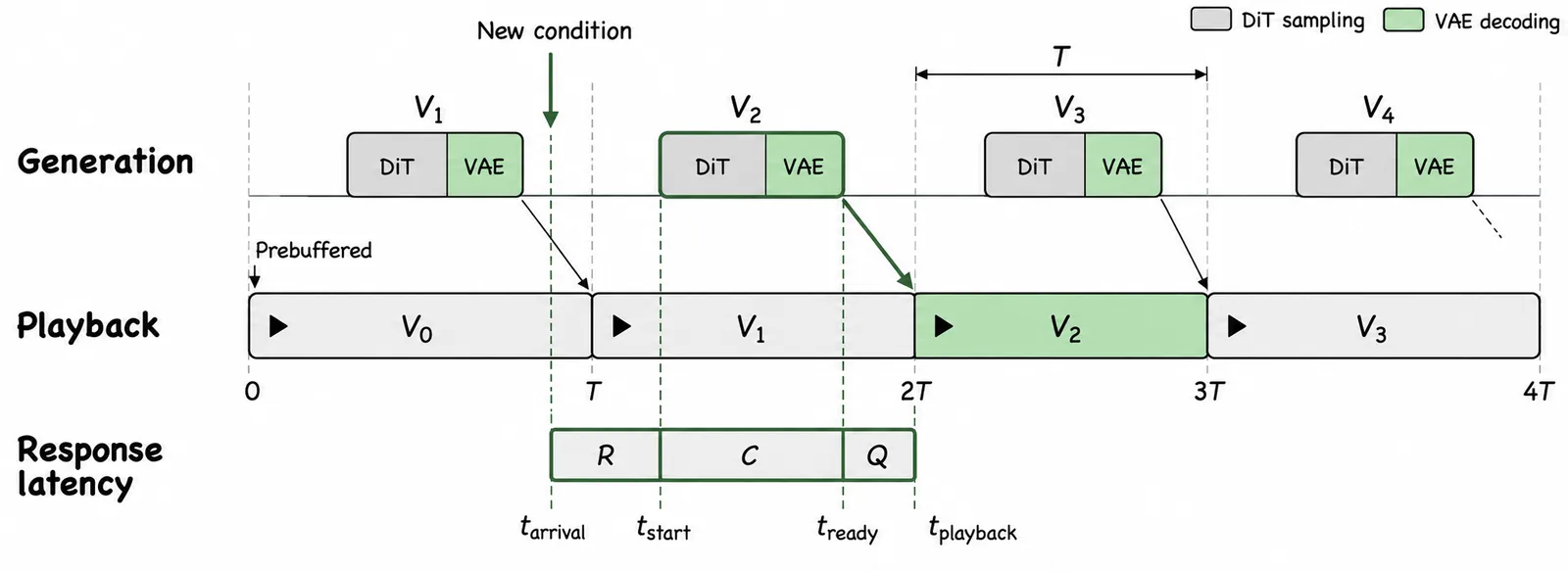
(Figure 2 in the paper) It draws the segment where, under a periodic reference schedule, one highlighted refresh waits $R$, then generates for $C$, then waits another $Q$ before being displayed. Each chunk is prepared against the next playback window, and the first window $V_0$ is pre-buffered. Since generation, even once finished, must wait until the playback boundary, response latency is not determined by generation time alone.
1.3 The Boundary Wait Remains Regardless of Generation Speed
Suppose that, as in existing schemes, the output reflecting a new condition can be put on screen only at fixed chunk playback boundaries. When generation time $C$ is fixed and arrival phases are uniform, the sum of the two waiting segments caused by alignment satisfies $E[R+Q] \ge T/2$, and therefore $E[L] \ge C + T/2$. (§3.4, Eq. (4); Appendix A.1 Proposition 1)
This lower bound needs to be read precisely. The bound concerns the average combined wait, not a per-request or per-component bound. $E[R+Q] \ge T/2$ is a lower bound on the sum, not on $E[R]$ and $E[Q]$ individually. Whether the waiting piles up before generation ($R$) or after generation ($Q$), the sum is the same. Also, the lower bound does not disappear even when generation time is zero.
1.4 A Small Example: Checking with Numbers
Let’s put the numbers in one by one. At 24 frames per second ($f=24$), if one latent frame represents 4 pixel frames ($r=4$), one latent frame covers $\delta = r/f = 4/24 \approx 0.17$ seconds. Taking the chunk as $K=4$ gives $T = K\delta \approx 0.67$ seconds, and alignment waits average $T/2 \approx 0.33$ seconds each. In other words, even if the DiT finishes in 0 seconds, the viewer waits 0.33 seconds on average.
(This is an illustrative assumption, not a measured figure from the paper. It is an arithmetic example blindly substituting into $T = Kr/f$, independent of the actual model’s $r$ and $f$.)
1.5 So Is Shrinking the Chunk the Answer?
The direct lever on the lower bound is shrinking $T = Kr/f$. With $r$ fixed, use a smaller $K$ or a higher temporal frame rate. But the paper’s preliminary experiments point the other way: larger chunk settings generally show better quality and also exploit GPU parallelism well, so sampling time increased only slightly while producing more latent frames. (§1, §4.2)
Here the paper’s central question emerges. Must the bidirectional modeling window be shrunk in order to gain reactivity. The answer is “no,” and instead of shrinking chunks, the convention of committing at chunk boundaries itself has to change.
2. Method: Speculative Sampling
2.1 Separating the Generation Unit from the Commit Unit
The key is to pull apart two sizes. How much the model predicts together in one shot ($K$, the generation unit), and how finely the system commits output at a time ($q$, the delivery unit). The delivery unit $q$ is the number of latent frames sent together, and this paper uses $q=1$. That is, it emits one latent frame at a time.
Thanks to this separation, “quality from the large window, reactivity from the small window” can be had at the same time.
2.2 Reusing Once-Computed Future, Swapping Only When Needed
The sequence of operations is as follows.
- Call the DiT once to jointly sample $K$ latent frames. Pad the 1 latent frame to be emitted next with $K-1$ noise latents, producing the $K$ latents together in a single bidirectional window. (§3.2, Eq. (2))
- Do not discard the predictions gained from the padding; store them in a prediction cache. A cache entry records the source/playout position correspondence and the condition version together, so it is managed independently of the state of subsequent calls.
- If the condition is unchanged, take the cache out as-is and play it in order. No additional sampling happens.
- If the condition changes, keep only the already-committed front part (the locked prefix), discard the not-yet-committed tail, and resample all $K$ latents wholesale under the new condition. The new sample is not made short to fit the remaining length of the old chunk.
- Committing the output is the act of making the content irreplaceable, and it can happen ahead of actual playback. A large chunk provides a reusable future, and the controller holds that future in a replaceable state until it is needed.
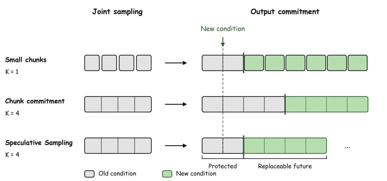
(Figure 1 in the paper) The three cases are compared side by side: small chunks ($K=1$), chunk-level commitment ($K=4$), and speculative sampling ($K=4$). Gray is the old condition and green is the new condition, and the bold green segment is the refreshed output. The dashed line marks the playback position at the moment the condition arrived; the “Protected” region is the irreversibly committed front part, and “Replaceable future” points to the replaceable rear part. The horizontal position represents the position in the video’s content, not computation time. That is, sampling happens jointly with a large chunk, and only the replaceable future beyond the protected prefix is swapped out.
2.3 Following a Small Example
Let $K=4$, $q=1$, and suppose one DiT call jointly creates latent frames 1·2·3·4.
| Time and input | Locked front part (committed, irreplaceable) | Prediction cache (replaceable) | Discarded | Output going to screen |
|---|---|---|---|---|
| One DiT call completed | (none) | 2, 3, 4 | (none) | 1 is decoded to pixels and played |
| 1 finished playing, new condition arrives while playing 2 | 1, 2 | resampling in progress (3, 4 invalidated) | 3, 4 | 2 (already committed, so played as-is) |
| Resampling with $K=4$ under the new condition completed | 1, 2 | 3′, 4′, 5′, 6′ | (none) | play 3′, then 4′ → 5′ → 6′ in order |
How to read it: 1 and 2 are committed and never erased; 3 and 4 are discarded the instant the new condition arrives and replaced with new values (3′, 4′); the new sample is always made as the full $K$ latents, never shortened to fit the old chunk’s remaining length. 5′ and 6′ are a future that no one has consumed yet, so if the condition changes again they too may be discarded.
(This is an illustrative example; the actual controller’s boundary/state decisions and details may differ.)
2.4 Orchestrating with the Two States, Produce and Consume
To run the above flow in a real system, what happens when must be pinned down. The paper turns this orchestration into an extended finite state machine (FSM). There are only two control states, and playback continues in both. (§3.2, Appendix C)
| State | What this state means | What actually happens in this state |
|---|---|---|
| Produce | One generation job is running | Calls the DiT to create $K$ latent frames, decodes completed latent frames with the VAE into pixels, and emits the ready batches at the assigned playback boundaries |
| Consume | No job is running | Takes the predictions remaining in the cache in order, plays them, converts them to pixels, and transmits them |
There are five kinds of events: condition arrival, output/state readiness, job completion, playback tick, and refill/retry wakeup. On each event the controller updates its registers, then checks whether an actionable branch boundary exists and decides whether to start a new job.
| Event | What the controller does | Effect on state |
|---|---|---|
| Condition arrival | Records only the pending condition version. It does not interrupt the running job. | Produce self-loop. If multiple pending updates exist, merge them into the latest version; discarded versions remain marked ‘superseded’ |
| Job completion | Validates the result and clears the slot | Stays in Produce if conditions for starting the next job exist, otherwise transitions to Consume |
| Playback tick | Plays the next ready batch and advances the playback cursor | Does not change state. The tick itself does not require DiT sampling |
| Update pending while idle | Among the positions after the locked prefix where the condition input is ready, the VAE continuity is valid, and the remaining playout deadline can be met, picks the earliest one and replaces only what follows it | Consume → Produce. Infeasible requests remain pending rather than discarding useful predictions |
| Refill condition met | Appends a new chunk when the remaining playable length falls short of the expected compute lead | Consume → Produce |
(While idle, update replanning and normal refill each start a job for separate reasons. The mere existence of a pending version does not by itself start a job.)
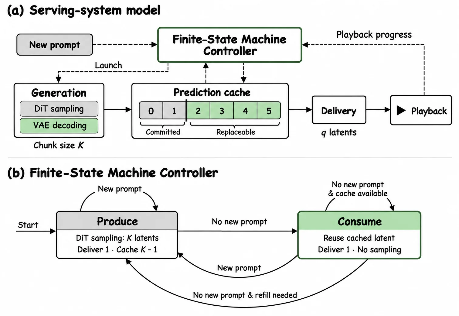
(Figure 3 in the paper) (a) shows the structure in which joint generation fills the prediction cache, and playback progress signals when it must be refilled. (b) is the FSM of the two states Produce (generating) and Consume (reusing predictions) when $q=1$. Condition updates do not stop the running generation but trigger only feasible replans, and playback continues in both states.
2.5 Attaching a Bidirectional Model to Streaming
A bidirectional generator typically provides an image·video-conditioned continuation interface. With a temporally compressing 3D VAE, this interface’s expectation of a ’temporally uncompressed first-frame latent’ collides with the fact that cached interior frames belong to a compressed group.
The paper decodes the held boundary to pixels, then re-encodes its last frame through the VAE’s first-frame path and hands it to the next DiT call. That matches the format the pretrained continuation interface expects. As an alternative, it mentions fine-tuning the model to accept compressed latent continuations directly. (§3.3)
2.6 What Disappears and What Remains
If, when a condition arrives, a prepared prefix is immediately available and there is no additional buffer constraint, the first display is aligned to a latent-frame boundary.
$$ t_{playback} = \delta \left\lceil \frac{t_{start} + C}{\delta} \right\rceil, \qquad Q = t_{playback} - (t_{start}+C), \qquad 0 \le Q < \delta $$In other words, alignment is bound not to the chunk ($T$) but to the delivery unit ($q=1$, one latent frame). (§3.4, Eq. (5))
Under ideal conditions, $E[L]$ comes down to $C + \delta/2$ (Appendix A.2). However, uniform arrivals do not guarantee uniform completion phases. If $R \ne 0$, $(t_{arrival}+R+C) \bmod \delta$ can cluster around particular values, so the actual $E[Q]$ is set by pipeline timing. This means only the alignment wait shrinks; the computation itself is unchanged.
What remains is generation and its residual wait. When one job fully occupies $C$ seconds per period $T$ ($C \le T$), that job must supply the prefix required by a new branch, and arrivals are uniform,
$$ E[R] = \frac{C^2}{2T}, \qquad E[L] = C + \frac{C^2}{2T} + E[Q] $$holds. (§3.4, Eq. (6), Appendix A.3)
Plugging the paper’s illustrative numbers $T=5$ s and $C=1.6$ s, the residual wait averages 0.256 s. Excluding $Q$, an idle-state arrival takes 1.6 s, an in-job arrival averages 2.4 s, and the unconditional average is 1.856 s. (A computed example, not a video-system measurement.)
The pivot this equation declares is clear. The responsiveness target moves from ‘shrinking the chunk ($T$)’ to ‘shrinking the generation time $C$ of the first output.’ The gains of DiT sampling acceleration and parallel acceleration are also measured through $C$ and the total resource cost.
2.7 The Cost, Recomputed
The claim is concrete on the cost side as well. If the condition does not change, predictions are reused, so in steady state the number of DiT sampling calls equals that of a matching chunk-unit baseline. Fine-grained delivery does not increase sampling. However, when little playable window remains, normal refill is still needed.
Only when the condition changes does extra work appear, equal to the discarded predictions. If each call produces $K$ useful latent groups at the same cost, and the fraction that ultimately fails to be played and gets discarded is $w$, then the relative DiT sampling workload is
$$ A \simeq \frac{1}{1-w} $$(§3.4, Eq. (7), Appendix B)
If updates are infrequent, this overhead is small. Appendix B.2’s independent-update model predicts that when the update probability is $p$, $A = \frac{Kp}{1-(1-p)^K}$, and for a Poisson arrival rate $\lambda$, if $\lambda T \ll 1$ then $A - 1 \simeq \frac{\lambda(T-\delta)}{2}$, that is, it drops. That said, $w$ depends not only on update frequency but also on chunk size and the chosen branch positions, and VAE decoding, adapter preparation, overlap truncation, interrupted jobs, and cache reconstruction require separate cost accounting.
3. Results
The experiments split into two layers. One is the effect of chunk size on quality and single forward time; the other is the end-to-end wait from condition arrival to screen display in actual serving. Since the two measure different things, they are examined separately. (§4)
One caveat. The forward-time profile in §4.1 is a shape-level measurement that includes communication and output collection but excludes text encoding, VAE decoding, and the sampler loop, and it differs from generation time $C$. (§4.1)
3.1 Chunk Size Is a Quality–Efficiency Trade-off
Wan1.3B was trained separately on Toy6K for each of $K \in \{1,3,7,21\}$ (1/2/4-step sampling) and evaluated with VBench on 81-frame, 16 fps video at 832×480 and 1280×720, over 946 prompts and 5 seeds. (§4.1)
At the same step count and resolution, $K>1$ generally earns higher VBench total scores than $K=1$.
| Steps / resolution | $K=1$ | $K=3$ | $K=7$ | $K=21$ |
|---|---|---|---|---|
| 4-step 480p | 79.00 | 81.66 | 81.70 | 82.13 |
| 4-step 720p | 78.84 | 81.59 | 81.86 | 81.65 |
(VBench total scores from the paper’s Table 1. The gain is not monotonically increasing, so the optimal $K$ differs per configuration. Quality was measured from models trained separately per chunk size.)
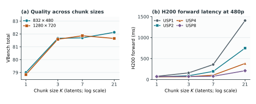
(Figure 5 in the paper) (a) plots Wan 4-step VBench total scores at resolutions 832×480 and 1280×720, and (b) H200 single-forward latency at 480p for USP1·2·4·8. Quality uses separately trained settings; timing uses a shared checkpoint and synthetic inputs.
At the same time, kernel forward time grows less than expected. Going from $K=1$ to $K=3$ triples the current chunk’s latent-frame count, but forward time grows only 2.05× at 480p and 2.74× at 720p.
| Resolution | $K$ | USP1 | USP2 | USP4 | USP8 |
|---|---|---|---|---|---|
| 480p | 1 | 77.5 | 63.7 | 65.9 | 72.1 |
| 480p | 3 | 159.2 | 91.5 | 67.0 | 72.9 |
| 480p | 7 | 358.3 | 194.7 | 105.2 | 78.6 |
| 480p | 21 | 1406.2 | 750.0 | 384.1 | 211.0 |
| 720p | 1 | 218.7 | 143.4 | 95.8 | 72.7 |
| 720p | 3 | 599.6 | 318.4 | 166.5 | 119.4 |
| 720p | 7 | 1521.4 | 809.2 | 443.8 | 276.4 |
| 720p | 21 | 6432.8 | 3335.5 | 1737.1 | 899.7 |
(The paper’s Table 2(a), H200 single forward in ms. Median of the slowest rank over 30 synchronized forwards, excluding 10 warmup runs.)
Growing parallelism enlarges the effect. 480p $K=7$ reaches 78.6ms at USP8, near USP1’s $K=1$ (77.5ms), and 720p $K=21$ falls from USP1’s 6432.8ms to USP8’s 899.7ms. That said, more GPUs are not always better (480p $K=1$ is faster at USP2, 63.7ms, than at USP8, 72.1ms). The right parallelism keeps large chunks efficient.
LTX-2.3 shows the same direction. $K \in \{1,3,9,15,45\}$ were each trained at 3 steps and evaluated on Internal32 (832×448, 24 fps, 361-frame output). The cached-forward of $K=45$ comes down from USP1’s 2016.2ms to USP8’s 507.9ms. However, LTX reports six VBench visual scores (subject consistency, background consistency, aesthetic quality, video quality, smoothness, dynamism) multiplied by 100 without a combined total, so a single-number “best $K$” cannot be read off for LTX. (The paper’s Table 2(b))
3.2 Large Chunks Are Also Fast in Real Serving
The comparison conditions must be fixed first. (§4.1)
- Wan1.3B: short/long chunks as K3/USP4 (4×B300) and K21/USP8 (8×B300), VAE on a separate GPU pipeline, 832×480.
- Sol-H3: 22·124-frame proposals, USP4/USP8 (4/8×B300), 832×480, 24 fps.
- LTX-2.3: short chunk as K3/USP1 (eager or CUDA Graph), long chunk as K15/USP2 (eager), 832×448, 24 fps, text·media on separate GPUs.
Within the same short/long setting, Baseline (commitment at chunk-boundary granularity) and speculative sampling share model placement, continuation interface, decoding, playback, and scheduling lead time. Each configuration is given thirty 60-second traces at a low frequency (1–2 updates per trace) and a high frequency (3–11 updates). L50/L95 are the 50th·95th percentiles (in seconds) of the ‘condition arrival→display’ response after clock alignment based on minimum RTT, and stall is the fraction (%) of the 60-second window occupied by playback underrun. LTX’s long-chunk implementation does not support CUDA Graph capture, so chunk-size comparison is on an eager basis.
Comparing the long-chunk setting by commitment scheme gives the following.
| Model (long chunk) | Scheme | Low-freq L50 / L95 | High-freq L50 / L95 |
|---|---|---|---|
| Sol-H3 | Baseline | 4.49 / 6.44 | 4.45 / 6.59 |
| Sol-H3 | Speculative sampling | 1.42 / 2.47 | 1.41 / 1.95 |
| Wan1.3B | Baseline | 3.23 / 4.64 | 3.11 / 4.66 |
| Wan1.3B | Speculative sampling | 1.32 / 1.91 | 1.35 / 1.63 |
| LTX-2.3 (eager) | Baseline | 4.82 / 6.99 | 5.09 / 6.98 |
| LTX-2.3 (eager) | Speculative sampling | 2.39 / 4.13 | 2.39 / 4.24 |
(Long-chunk rows from the paper’s Table 3. All at 480p-class.)
Across all three models, speculative sampling in long chunks brought L50 down to less than half of baseline’s.
Headroom also appears alongside. The per-GPU kernel activity rate (time-weighted average) drops sharply in the long setting — Wan 17–20% (short chunks 50–52%), Sol-H3 18–23% (short chunks 49–50%) — while LTX eager sits at 21–25%, similar to its short chunks (22–23%). This idle reads as room to serve more concurrent streams. The activity-rate increase at high-frequency updates is somewhat larger, but the long setting stays within 20–25%. The measurement scope differs per model: Wan counts only the DiT GPUs, while LTX includes the text·media GPUs.
The most striking result is Sol-H3. Using speculative sampling on long chunks, L50 lands at 1.42/1.41 s at low/high frequency, below the small-chunk baseline’s 1.87/1.87 s, while playback stall is also 0.000%. A direct demonstration that keeping a large bidirectional window is not the path of giving up reactivity.
Cases where playback stalls stand out in LTX. LTX’s short-chunk eager run measured playback underrun at 19.669% at low frequency and 20.339% at high frequency. Switching to the CUDA Graph variant brings the baseline down to 0.005%/0.021%, but speculative sampling in the same variant remains at 1.781%/4.407%. In long chunks, Baseline stays low at 0.069%/0.065% and speculative sampling at 0.204%/0.524%. In short eager, baseline and speculative sampling were both similar at around the late-19% range, so in this run mode the commitment scheme made little difference to stall.
3.3 Predictions Match Measurement
Overlaying the mean response reduction onto theory, the boundary-wait model can be seen to actually work. Sol-H3’s measured reduction is 0.493/2.814 s in the short/long settings, close to the theoretical predictions of 0.438/2.562 s. The tendency for the reduction to grow with chunk size also matches the prediction. Wan went 0.155 → 1.744 s and LTX eager 0.014 → 2.116 s, following the prediction that ’the larger the chunk, the more boundary wait there is to remove.’ (§4.3)
There is one more summary figure. With speculative sampling applied, the long setting’s L50 stops at a level 0.26–0.39 s above the same model’s short setting (all three models, both request loads). In other words, even with large chunks, the reactivity loss is effectively suppressed to the 0.3 s level.
4. Limitations and When to Use It
The limitations the authors themselves admit are two.
First, predictions only pay when they are reused before the new condition invalidates them. If updates are frequent or continuous, much of a chunk is discarded and DiT compute is wasted. $w$ depends not only on update frequency but also on chunk size and the chosen branch positions.
Second, because of bidirectional attention within a chunk, the retained KV can carry information about later content that is later discarded. Even after KV entries are deleted, that influence can remain in the regenerated continuation. (§5)
Adding from a reviewer’s perspective, there are several constraints.
- The update frequencies the experiments cover are only two ranges, 1–2 and 3–11 per 60-second trace. A situation where the viewer manipulates the screen continuously has not been validated.
- L50/L95 measure ‘from condition arrival to display.’ The moment the condition’s effect becomes perceptible — the semantic response — is left to separate measurement (Appendix D).
- Separately instrumented values of $R$ and $Q$ in actual deployment, and the measured value of the rate $w$ at which prediction reuse actually happens, are not reported in the original (not reported). $A \simeq 1/(1-w)$ is an accounting identity over sampling calls, not a measured value of $w$.
- The results are confirmed at specific chunk·resolution·GPU configurations of three models, so it is hard to assert they hold as-is under other frame rates, VAEs, and backbones. The added cost of the VAE first-frame-path re-encoding is also a separate cost-accounting item.
When it is worth using in an operating environment can be read from this analysis. It fits scenarios with intermittent updates — for example, commands changing occasionally within a scene (the experiment traces also change actions within a scene) — best. It is also promising when you want to serve a large bidirectional model for streaming without continued training. Conversely, when the condition keeps changing, or when GPU headroom is lacking so that $C$ approaches $T$, the benefit shrinks. In the limiting case $C=T$, the generation worker is always busy, so $E[R]=T/2$ and $Q=0$, and the mean $L$ remains $3T/2$, equal to the fixed-chunk-boundary baseline (Appendix A.3). Fine-grained delivery alone does not improve it.
In the end, this method shifts the design’s center of gravity. It lifts the fixed constraint that chunk size must be shrunk, and instead restores chunk size as a decision variable that jointly controls quality and reactivity. The center of gravity of optimization moves to $C$, the remaining bottleneck: shrinking the generation time of the first output.
Tables from the paper
Tables converted mechanically from the arXiv e-print LaTeX source. The numbers are the paper’s own and did not pass through a model.
Table 1. Wan1.3B quality measurements. Total is the reported VBench aggregate, with its quality and semantic components; the table also includes dynamic degree, VisionReward, and instruction following.
| Resolution | Steps | $K$ | Total | Quality | Semantic | Dynamic | VisionReward | Instruction |
|---|---|---|---|---|---|---|---|---|
| 480p | 1 | 1 | 79.11 | 81.80 | 68.34 | 4.00 | 6.50 | 90.00 |
| 1 | 3 | 80.38 | 83.40 | 68.29 | 58.00 | 4.81 | 94.00 | |
| 1 | 7 | 81.35 | 83.97 | 70.86 | 48.00 | 5.79 | 100.00 | |
| 1 | 21 | 81.68 | 84.83 | 69.08 | 85.00 | 9.93 | 94.00 | |
| 2 | 1 | 80.07 | 82.76 | 69.34 | 14.00 | 9.31 | 98.00 | |
| 2 | 3 | 81.62 | 84.63 | 69.57 | 57.00 | 9.82 | 100.00 | |
| 2 | 7 | 80.84 | 84.06 | 67.94 | 93.00 | 9.29 | 100.00 | |
| 2 | 21 | 81.84 | 84.62 | 70.74 | 71.00 | 10.17 | 100.00 | |
| 4 | 1 | 79.00 | 81.38 | 69.50 | 13.00 | 7.65 | 96.00 | |
| 4 | 3 | 81.66 | 84.70 | 69.51 | 80.00 | 9.64 | 100.00 | |
| 4 | 7 | 81.70 | 84.73 | 69.56 | 78.00 | 10.19 | 98.00 | |
| 4 | 21 | 82.13 | 85.03 | 70.54 | 85.00 | 9.66 | 98.00 | |
| 720p | 1 | 1 | 78.94 | 81.37 | 69.19 | 4.00 | 5.82 | 92.00 |
| 1 | 3 | 79.99 | 82.70 | 69.18 | 47.00 | 3.93 | 98.00 | |
| 1 | 7 | 80.78 | 83.05 | 71.67 | 41.00 | 5.23 | 96.00 | |
| 1 | 21 | 80.49 | 83.10 | 70.04 | 67.00 | 9.56 | 100.00 | |
| 2 | 1 | 79.86 | 82.40 | 69.70 | 9.00 | 9.43 | 98.00 | |
| 2 | 3 | 81.52 | 84.11 | 71.18 | 48.00 | 10.10 | 100.00 | |
| 2 | 7 | 80.97 | 83.79 | 69.67 | 84.00 | 9.25 | 94.00 | |
| 2 | 21 | 80.26 | 82.61 | 70.84 | 39.00 | 9.91 | 98.00 | |
| 4 | 1 | 78.84 | 81.19 | 69.44 | 22.00 | 7.18 | 92.00 | |
| 4 | 3 | 81.59 | 84.36 | 70.49 | 74.00 | 9.59 | 100.00 | |
| 4 | 7 | 81.86 | 84.62 | 70.83 | 73.00 | 9.77 | 96.00 | |
| 4 | 21 | 81.65 | 84.43 | 70.52 | 66.00 | 9.36 | 96.00 |
Table 2. H200 single-forward profiles and LTX quality. Wan timings use one shared reference checkpoint across nominal step configurations; LTX timings are cached-forward measurements for each $(K,\mathrm{USP})$. LTX uses three steps. SC/BC denote subject/background consistency; visual scores are multiplied by 100 without a combined total.
| (a) Wan H200 forward (ms) | |||||
|---|---|---|---|---|---|
| tabularllrrrr Resolution | $K$ | USP1 | USP2 | USP4 | USP8 |
| 480p | 1 | 77.5 | 63.7 | 65.9 | 72.1 |
| 3 | 159.2 | 91.5 | 67.0 | 72.9 | |
| 7 | 358.3 | 194.7 | 105.2 | 78.6 | |
| 21 | 1406.2 | 750.0 | 384.1 | 211.0 | |
| 720p | 1 | 218.7 | 143.4 | 95.8 | 72.7 |
| 3 | 599.6 | 318.4 | 166.5 | 119.4 | |
| 7 | 1521.4 | 809.2 | 443.8 | 276.4 | |
| 21 | 6432.8 | 3335.5 | 1737.1 | 899.7 |
Table 3. Online serving results at 480p class for Wan1.3B, LTX-2.3, and Sol-H3. Baseline denotes chunk-level commitment; Speculative Sampling denotes our method. LTX’s parenthesized CUDA Graph configurations apply graph capture and replay to the DiT; Long versus Short isolates chunk size among eager configurations, while parenthesized versus unparenthesized Short isolates this execution mode. $L_{50}/L_{95}$ are seconds; GPU kernel activity and stall ratio are percentages. GPU is the time-weighted mean over the monitored deployment GPUs, with model-specific scope described in the text.
| Model | Resolution | Configuration | Low-frequency updates $L_{50}$ | Low-frequency updates $L_{95}$ | Low-frequency updates GPU | Low-frequency updates Stall | High-frequency updates $L_{50}$ | High-frequency updates $L_{95}$ | High-frequency updates GPU | High-frequency updates Stall |
|---|---|---|---|---|---|---|---|---|---|---|
| Wan1.3B | 480p | Short-Baseline | 1.13 | 1.47 | 49.67 | 0.000 | 1.24 | 1.65 | 52.19 | 0.000 |
| Long-Baseline | 3.23 | 4.64 | 16.97 | 0.000 | 3.11 | 4.66 | 17.29 | 0.000 | ||
| Short–Speculative Sampling | 1.01 | 1.14 | 50.45 | 0.000 | 1.05 | 1.35 | 52.25 | 0.000 | ||
| Long–Speculative Sampling | 1.32 | 1.91 | 17.28 | 0.000 | 1.35 | 1.63 | 19.92 | 0.000 | ||
| LTX-2.3 | 480p | Short-Baseline | 2.12 | 2.58 | 22.02 | 19.669 | 2.01 | 2.64 | 22.69 | 20.339 |
| Short-Baseline (CUDA Graph) | 1.81 | 2.32 | 29.19 | 0.005 | 1.89 | 2.34 | 30.30 | 0.021 | ||
| Long-Baseline | 4.82 | 6.99 | 20.47 | 0.069 | 5.09 | 6.98 | 21.41 | 0.065 | ||
| Short–Speculative Sampling | 2.00 | 2.67 | 21.94 | 19.758 | 2.00 | 2.57 | 22.76 | 19.878 | ||
| Short–Speculative Sampling (CUDA Graph) | 2.01 | 2.82 | 29.03 | 1.781 | 1.94 | 2.54 | 29.99 | 4.407 | ||
| Long–Speculative Sampling | 2.39 | 4.13 | 21.29 | 0.204 | 2.39 | 4.24 | 24.51 | 0.524 | ||
| Sol-H3 | 480p | Short-Baseline | 1.87 | 2.11 | 48.62 | 0.000 | 1.87 | 2.04 | 49.10 | 0.000 |
| Long-Baseline | 4.49 | 6.44 | 17.42 | 0.000 | 4.45 | 6.59 | 18.25 | 0.000 | ||
| Short–Speculative Sampling | 1.11 | 1.50 | 48.85 | 0.000 | 1.15 | 1.53 | 50.00 | 0.000 | ||
| Long–Speculative Sampling | 1.42 | 2.47 | 18.45 | 0.000 | 1.41 | 1.95 | 22.67 | 0.000 |
Figures in this post are taken from the original arXiv:2610.20556 (CC BY 4.0). Only size and format were changed.
Comments