Training on long documents across several GPUs creates more than a compute problem. Each GPU also needs the right attention mask: the rules that determine which tokens may attend to which other tokens. If those rules leave one GPU with more work than the others, the entire training step waits for it.
FlashMask-3 starts with how masks are stored, then uses that representation to select work, distribute it, and overlap communication with computation. The paper reports a 7.3–11.0% improvement in full training throughput for a MoE model with a 128K context on 128 H100 GPUs. That result must be distinguished from the speedup of the attention kernel alone (§4.3, Table 1).
Splitting a long sequence also creates a mask problem
Attention computes how much information each token takes from other tokens. A mask rules out relationships that are not allowed. For example, when several documents are packed into one input, tokens from different documents can be prevented from attending to each other. Sliding-window attention, which only allows nearby tokens, is another example.
Representing a mask as a large table becomes expensive. With $n$ tokens there are $n^2$ token pairs, so storing and processing the mask grows costly as the input gets longer. The earlier FlashMask reduces storage to $O(n)$ by representing structured masks with interval boundaries (§2.2).
Using several GPUs adds another challenge. Context Parallelism (CP) distributes attention work for a long sequence across GPUs. Each GPU needs a mask for its assigned tokens, and equal token counts do not imply equal amounts of computation. Simply splitting the sequence into equally sized pieces does not guarantee balanced work (§2.3).
FlashMask-3 connects these two problems. It aims to use compressed masks efficiently inside a GPU kernel while preventing mask processing and communication from becoming bottlenecks when work is distributed across GPUs.
Store boundaries instead of a large table
In an attention matrix, rows correspond to queries, the tokens requesting information, and columns to keys, the tokens being attended to. FlashMask stores the query intervals that are masked out for each key. For masks that fit this representation, each key requires at most two masked intervals, or four boundary values (§2.2).
A small example shows why this helps construct per-GPU masks. This is an illustrative example, not a measurement from the paper.
Suppose eight tokens are split across two GPUs, and the masked query interval for one key is $[6,8)$ in global coordinates. GPU A handles queries 0–3, while GPU B handles queries 4–7.
| GPU | Assigned global query interval | Overlap with masked interval | GPU-local coordinates |
|---|---|---|---|
| A | $[0,4)$ | None | Empty interval |
| B | $[4,8)$ | $[6,8)$ | $[2,4)$ |
GPU B only needs to subtract its starting offset, 4. GPU A clips the out-of-range boundaries to the end of its range, obtaining an empty interval. If both already know the global boundaries and their own assignments, they need no communication to perform this conversion.
The paper extends this idea to cases where one GPU owns several noncontiguous chunks. It clips boundaries to the assigned chunks, shifts them into local coordinates, and merges them with a maximum operation. Theorem 1 establishes that this conversion preserves the original masking relationships (§3.2, Appendix C.1).
Here, zero communication refers only to converting mask boundaries into local coordinates. GPUs still need to exchange key and value data for attention computation.
Reuse the boundaries to choose and distribute work
Compact mask storage alone does not make a GPU fast. FlashMask-3 uses the same boundaries to skip unnecessary work and distribute the remaining work more evenly.
Filter blocks before computing them
The GPU kernel processes the attention matrix in small blocks. If an entire block is masked, it needs neither a data load nor a matrix multiplication. A partially masked block still needs computation with masking applied.
FlashMask-3’s KV Index Generator identifies these cases and produces a list of blocks to compute. The loader fetches blocks from that list, while the matrix-multiplication threads concentrate on computation. This separates mask inspection from the main compute path while using Hopper’s asynchronous data transfers (TMA) and matrix-multiplication instructions (WGMMA) (§3.1).
A simple porting experiment illustrates why this separation matters. For a 128K Document mask, forward throughput was 19.0 TFLOPs/s for a FA3-style Hopper port without the KV Index Generator, versus 577.6 TFLOPs/s for the complete FlashMask-3 implementation. The full implementation includes other optimizations, however, so the entire difference cannot be attributed to this component alone (Appendix D.4, Table 7).
Balance actual computation rather than token counts
Two equally long chunks can require different amounts of work if one has more masked blocks. FlashMask-3’s HCC-IPO algorithm accounts for that difference. It first balances computation across GPUs, adjusts assignments to reduce cross-node transfers, then rebalances within each node (§3.3).
A similar imbalance can occur inside one GPU: some execution units finish early while others remain occupied. The PPT scheduler lets a GPU thread block take another task when it finishes its current one. These two scheduling mechanisms reduce waiting across GPUs and within each GPU, respectively (§3.1).
Overlap necessary communication with computation
Even with context parallelism, each GPU needs key and value data held by other GPUs. FlashMask-3 skips transfers of chunks that the mask makes entirely unnecessary and separates inter-node and intra-node communication routes. During backward computation, it divides work into segments so that communication for one segment overlaps computation for the next (§3.4).
Overall pipeline
Saying “the mask is a bottleneck” combines three operations: building a large table of masked entries, selecting blocks to compute, and assigning work to GPUs. Slow preparation or uneven assignments can delay the next training step.
The figure uses small illustrative examples to make those operations visible. Its three panels are independent examples, not performance measurements from the paper.
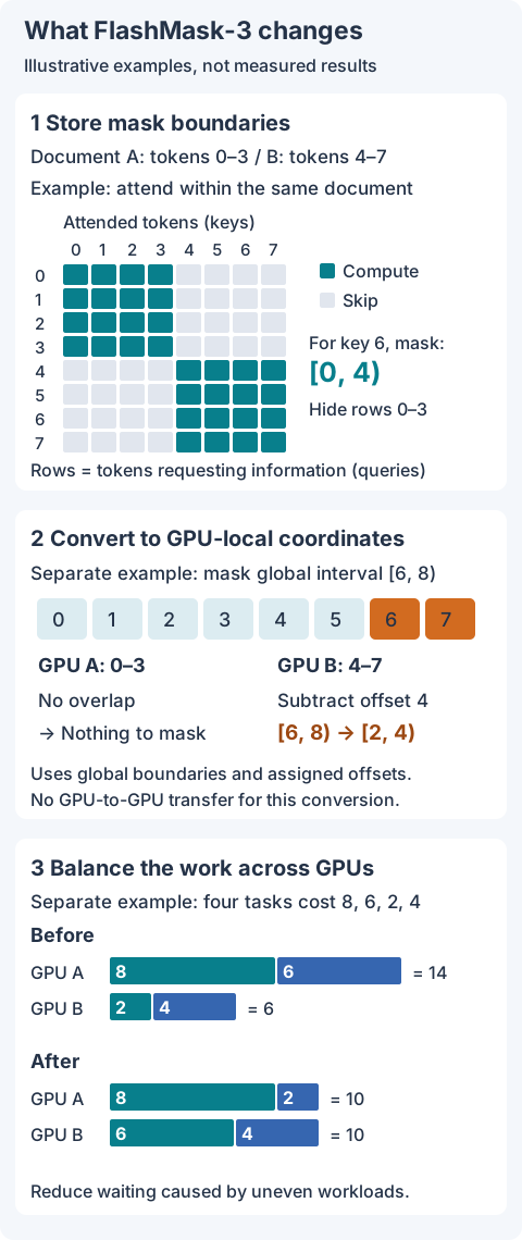
In the first panel, green entries are token pairs to compute; gray entries can be skipped. For key 6, rows 0–3 are masked, which can be recorded as the interval [0, 4). The kernel uses such boundaries to avoid loading or computing fully masked blocks (§2.2, §3.1).
The second panel converts boundaries into GPU-local coordinates. Global interval [6, 8) becomes [2, 4) on GPU B. This conversion needs no communication between GPUs, but attention still requires key and value data transfers (§3.2).
In the third panel, assigning the same number of tasks to each GPU produces costs of 14 and 6. Reassigning the tasks yields 10 each. The actual HCC-IPO also considers cross-node transfer costs. The change from 14 to 10 uses arbitrary illustrative work units, not measured speedups (§3.3).
Finally, necessary transfers overlap computation. For example, the system can fetch data for a subsequent segment while computing a ready segment, reducing waiting. The figure shows storage, coordinate conversion, and assignment; it does not depict the detailed communication-overlap implementation (§3.4).
How much faster is actual training?
The most useful result to examine first is full training throughput. Faster attention can produce a smaller overall gain when other training operations remain unchanged.
The experiment trained a MoE model with 118B total and 14B active parameters at a 128K context length. It used 128 H100 GPUs, CP degree 16, and an 8K local sequence per GPU. The baseline below already uses the FlashMask-3 kernel, but retains Dual Chunk assignment and all-gather communication with the proposed balancing and overlap disabled. This table therefore measures the additional benefit of distributed execution optimizations, rather than simply replacing the attention kernel (§4.3, Table 1).
| Mask sparsity | Baseline throughput | FlashMask-3 throughput | Full training gain | Attention forward+backward gain |
|---|---|---|---|---|
| 70% | 712.6 tokens/s/GPU | 764.7 tokens/s/GPU | 7.3% | 24.5% |
| 80% | 753.3 tokens/s/GPU | 811.4 tokens/s/GPU | 7.7% | 42.1% |
| 86% | 812.4 tokens/s/GPU | 902.1 tokens/s/GPU | 11.0% | 44.9% |
The table reproduces the paper’s mean values. Standard deviations and component-level experiments are available in the collapsed source tables below.
The distinction between the final two columns matters. Attention computation improved by up to 44.9%, but full training throughput improved by up to 11.0%. Training also includes operations this method does not change, such as gradient synchronization and optimizer updates. Reading the result as “44.9% faster training” would misstate its scope.
In a separate distributed attention experiment, total forward+backward throughput was 1.09–1.46 times that of MagiAttention. That experiment kept the local sequence length at 8K per GPU while varying CP degree from 4 to 32. Its results should not be treated as the same metric as full training throughput above (§4.2, Table 5).
Does FlashMask-3 beat FlashAttention-3 on one GPU? Not for the five masks compared in Table 6: its throughput was 0.71–1.00 times FA3’s. Its value lies in supporting a broader range of structured masks alongside distributed execution, rather than winning every FA3 comparison (Appendix D.4).
Limitations to check before adoption
The first question is whether the mask fits this representation. If the masked queries for a key cannot be expressed as two intervals, the current format cannot be used directly. The kernel also targets Hopper’s TMA and WGMMA facilities; matching these gains on another GPU requires implementation work and validation. Both are limitations acknowledged by the authors (Appendix A).
The communication optimizations also depend on hardware layout. They exploit fast intra-node NVLink and slower inter-node links, and hierarchical routing currently applies to forward all-gather. Other topologies and an extension to backward reduce-scatter need further validation (Appendix A, C.4).
From a reviewer’s perspective, assignment overhead deserves attention too. The paper precomputes scheduling decisions and prefetches them to hide their cost during execution. If masks change too often to reuse this preparation, the benefit may shrink. In Figure 7(b), IPO’s load-balance advantage over the simpler LPT is only about 0.01 where it improves the result. Whether that extra scheduling complexity is useful for a particular workload needs separate evaluation (§4.4, Appendix D.5).
The scope of quality validation also matters. The mask conversion preserves the original masking relationships, and the paper compares training losses across 1,581 steps. It does not provide a separate downstream benchmark evaluation (Theorem 1, Appendix D.3).
FlashMask-3 is worth examining when long documents, structured masks, and multi-GPU training on Hopper are all required. Its central contribution is to use mask boundaries as information for deciding actual computation and communication, beyond merely storing the mask compactly. An adoption assessment should check mask compatibility, GPU and network layout, then full training throughput.
Expand all 8 tables from the paper
Tables converted mechanically from the arXiv e-print LaTeX source. The numbers are the paper’s own and did not pass through a model.
Table 1. End-to-end training throughput of a 118B-A14B MoE model (128K context, CP degree 16, $S_{\text{local}}{=}8$K tokens per device, $H_q{=}64$, $H_{kv}{=}8$, document mask) on 128 H100 GPUs, for three datasets of differing average mask sparsity. Each run covers 70 steps; we discard the 10 highest and 10 lowest throughput steps and report the mean ± one standard deviation over the remaining 50. $\Delta_{\text{attn}}$ is the corresponding attention forward+backward speedup over the baseline.
| Configuration | 70% sparsity tokens/s/GPU | 70% sparsity $\Delta_{\text{attn}}$ | 80% sparsity tokens/s/GPU | 80% sparsity $\Delta_{\text{attn}}$ | 86% sparsity tokens/s/GPU | 86% sparsity $\Delta_{\text{attn}}$ |
|---|---|---|---|---|---|---|
| Baseline (Dual Chunk + all-gather) | 712.6 ± 8.7 | – | 753.3 ± 34.7 | – | 812.4 ± 57.1 | – |
| + HCC-IPO balancing | 732.2 ± 24.5 | +10.4% | 786.2 ± 65.2 | +19.1% | 858.5 ± 62.1 | +10.5% |
| + mask-aware overlap | 750.8 ± 6.4 | +15.9% | 785.0 ± 33.6 | +13.9% | 860.0 ± 55.0 | +20.5% |
| + both, hierarchical routing off | 700.6 ± 28.8 | +8.4% | 742.0 ± 72.6 | +21.5% | 828.0 ± 60.6 | +23.2% |
| + both, w/o chunk-skip pruning | 750.0 ± 20.6 | +20.5% | 788.4 ± 55.0 | +25.4% | 888.6 ± 69.6 | +27.9% |
| FlashMask-3 (balance + overlap) | 764.7 ± 28.8 | +24.5% | 811.4 ± 75.9 | +42.1% | 902.1 ± 72.6 | +44.9% |
Table 2. Resource profile of the FlashMask-3 distributed mask preprocessing on rank $r$ owning $n_r$ chunks. $N_K$ denotes the global key length. All operations are elementwise and parallelized over the key dimension.
| Operation | Time | Memory | Cross-rank comm. | Kernel interface |
|---|---|---|---|---|
| Single-chunk clip (Def. ) | $O(N_K)$ | $O(N_K)$ | 0 | shared |
| Multi-chunk shift+merge (Def. ) | $O(n_r N_K)$ | $O(N_K)$ | 0 | shared |
| Total mask preprocessing | $O(n_r N_K)$ | $O(N_K)$ | 0 | shared |
Table 3. IPO phase ablation across representative CP configurations. Subopt: fraction of random instances not matching the optimum. Max gap: worst-case relative excess over optimal makespan. P3 wins: cases where Phase 3 improves upon Phase 2. All configurations use 200 random instances (100 for $N\!=\!128$).
| Configuration | $(N,P,\kappa,w_{\max})$ | LPT Subopt | LPT Gap | LPT+P2 Subopt | LPT+P2 Gap | LPT+P2+P3 Subopt | LPT+P2+P3 P3 wins |
|---|---|---|---|---|---|---|---|
| Uniform | $(64,16,4,10^3)$ | 99.0% | 6.54% | 86.0% | 6.29% | 0% | 172 |
| Uniform (wide) | $(64,16,4,10^4)$ | 100% | 8.67% | 93.5% | 3.42% | 0% | 187 |
| Causal | $(64,8,8,200)$ | 93.5% | 2.51% | 53.5% | 1.39% | 0% | 107 |
| Uniform$^\dagger$ | $(128,16,8,200)$ | 85.0% | 1.08% | 48.0% | 0.79% | 0% | 48 |
Table 4. FlashMask-3 throughput improvement over baselines (forward+backward TFLOPs/s). Reported as $(T_{\text{ours}} / T_{\text{baseline}} - 1) \times 100\%$.
| Baseline | Scope | Min | Max | Mean |
|---|---|---|---|---|
| FlexAttention | All | +33.6% | +70.5% | +55.3% |
| 8K | +33.6% | +62.9% | +50.6% | |
| 128K | +51.9% | +70.0% | +58.9% | |
| Magi-Attention | All | +2.0% | +44.1% | +15.0% |
| 8K | +12.0% | +44.1% | +25.0% | |
| 128K | +2.0% | +8.9% | +5.9% | |
| FlashMask | All | +44.9% | +140.5% | +82.6% |
| 8K | +44.9% | +84.8% | +66.2% | |
| 128K | +74.4% | +140.5% | +97.3% |
Table 5. FlashMask-3 speedup over distributed baselines (aggregated over all masks $\times$ CP sizes).
| vs. Baseline | Phase | Min | Max | Geo.\ Mean ± std |
|---|---|---|---|---|
| MagiAttention | FWD | 1.04$\times$ | 2.39$\times$ | 1.56 ± 0.53$\times$ |
| BWD | 1.10$\times$ | 1.19$\times$ | 1.15 ± 0.03$\times$ | |
| Total | 1.09$\times$ | 1.46$\times$ | 1.26 ± 0.15$\times$ | |
| Megatron Ring | FWD | 1.62$\times$ | 4.12$\times$ | 2.50 ± 0.97$\times$ |
| BWD | 1.86$\times$ | 3.57$\times$ | 2.38 ± 0.56$\times$ | |
| Total | 1.80$\times$ | 3.71$\times$ | 2.42 ± 0.65$\times$ | |
| Megatron AllGather | FWD | 1.31$\times$ | 2.24$\times$ | 1.57 ± 0.31$\times$ |
| BWD | 1.85$\times$ | 3.15$\times$ | 2.21 ± 0.43$\times$ | |
| Total | 1.71$\times$ | 2.92$\times$ | 2.05 ± 0.39$\times$ |
Table 6. Single-GPU throughput on five masks supported by FA3 (total forward$+$backward TFLOPs/s, mean ± std over 50 iterations). Parentheses give the ratio to FA3.
| Seq | Mask | FA3 | FlashMask-3 | FlexAttention | MagiAttention |
|---|---|---|---|---|---|
| 8K | Full | 604.43 ± 1.27 | 569.84 ± 1.88 (0.94) | 394.15 ± 1.34 (0.65) | 513.66 ± 8.95 (0.85) |
| 8K | Causal | 579.73 ± 0.35 | 520.85 ± 0.54 (0.90) | 341.68 ± 1.45 (0.59) | 482.17 ± 1.71 (0.83) |
| 8K | Sliding Window | 407.23 ± 1.54 | 290.30 ± 1.04 (0.71) | 218.93 ± 1.73 (0.54) | 166.22 ± 0.15 (0.41) |
| 8K | Causal Document | 478.96 ± 27.20 | 377.86 ± 35.26 (0.79) | 264.06 ± 18.37 (0.55) | 247.92 ± 47.43 (0.52) |
| 8K | Document | 546.29 ± 17.93 | 460.49 ± 31.77 (0.84) | 299.46 ± 26.68 (0.55) | 352.82 ± 48.32 (0.65) |
| 32K | Full | 616.65 ± 0.65 | 603.63 ± 1.48 (0.98) | 408.22 ± 0.02 (0.66) | 593.40 ± 1.30 (0.96) |
| 32K | Causal | 611.66 ± 0.59 | 587.87 ± 0.88 (0.96) | 371.48 ± 0.47 (0.61) | 563.30 ± 3.20 (0.92) |
| 32K | Sliding Window | 534.47 ± 1.71 | 465.00 ± 0.68 (0.87) | 309.52 ± 2.77 (0.58) | 378.13 ± 0.81 (0.71) |
| 32K | Causal Document | 532.68 ± 6.32 | 435.54 ± 15.28 (0.82) | 294.92 ± 8.42 (0.55) | 328.81 ± 21.48 (0.62) |
| 32K | Document | 592.03 ± 5.04 | 503.66 ± 6.68 (0.85) | 312.10 ± 19.68 (0.53) | 431.37 ± 17.05 (0.73) |
| 128K | Full | 603.12 ± 1.14 | 602.06 ± 0.92 (1.00) | 415.16 ± 0.40 (0.69) | 595.04 ± 2.00 (0.99) |
| 128K | Causal | 618.52 ± 0.48 | 587.92 ± 1.33 (0.95) | 377.21 ± 0.01 (0.61) | 580.09 ± 0.34 (0.94) |
| 128K | Sliding Window | 592.51 ± 0.46 | 561.46 ± 1.40 (0.95) | 358.07 ± 0.40 (0.60) | 514.87 ± 2.36 (0.87) |
| 128K | Causal Document | 591.87 ± 3.64 | 542.68 ± 6.73 (0.92) | 352.92 ± 3.70 (0.60) | 498.60 ± 8.79 (0.84) |
| 128K | Document | 615.62 ± 1.85 | 575.86 ± 4.11 (0.94) | 367.07 ± 7.90 (0.60) | 546.12 ± 3.83 (0.89) |
Table 7. Isolating the warp specialization from the Hopper port (forward TFLOPs/s, mean ± std). Parentheses give the ratio to FlashMask-3.
| Seq | Mask | FlashMask-3 | FlashMask | FA3-style Hopper port |
|---|---|---|---|---|
| 8K | Full | 596.53 ± 2.26 | 384.88 ± 1.84 (0.65) | 214.01 ± 0.23 (0.36) |
| 8K | Causal | 553.31 ± 1.13 | 373.46 ± 1.37 (0.67) | 241.86 ± 0.13 (0.44) |
| 8K | Sliding Window | 432.15 ± 6.60 | 256.63 ± 0.07 (0.59) | 35.77 ± 0.07 (0.08) |
| 8K | Causal Document | 483.97 ± 29.40 | 302.03 ± 15.27 (0.62) | 64.77 ± 15.83 (0.13) |
| 8K | Document | 532.26 ± 24.90 | 287.89 ± 34.54 (0.54) | 55.03 ± 14.14 (0.10) |
| 32K | Full | 614.19 ± 1.15 | 388.92 ± 1.84 (0.63) | 214.22 ± 0.08 (0.35) |
| 32K | Causal | 593.97 ± 0.87 | 379.46 ± 1.65 (0.64) | 244.95 ± 0.14 (0.41) |
| 32K | Sliding Window | 553.66 ± 2.78 | 274.60 ± 0.54 (0.50) | 31.20 ± 0.08 (0.06) |
| 32K | Causal Document | 515.48 ± 10.22 | 256.39 ± 9.50 (0.50) | 25.29 ± 2.81 (0.05) |
| 32K | Document | 544.56 ± 5.93 | 191.12 ± 36.15 (0.35) | 21.42 ± 2.48 (0.04) |
| 128K | Full | 613.49 ± 2.15 | 390.66 ± 0.19 (0.64) | 211.51 ± 0.53 (0.34) |
| 128K | Causal | 544.83 ± 0.55 | 359.79 ± 0.52 (0.66) | 245.99 ± 0.02 (0.45) |
| 128K | Sliding Window | 573.63 ± 0.94 | 274.44 ± 0.67 (0.48) | 29.96 ± 0.01 (0.05) |
| 128K | Causal Document | 554.50 ± 9.57 | 252.96 ± 9.03 (0.46) | 22.15 ± 2.44 (0.04) |
| 128K | Document | 577.55 ± 3.33 | 217.27 ± 40.17 (0.38) | 18.97 ± 2.08 (0.03) |
Table 8. Standalone scheduling latency against attention time ($P{=}32$, chunk 2048).
| Mask | Attention (ms) | Schedule (ms) |
|---|---|---|
| Causal Document | 35.08 ± 4.19 | 42.75 ± 8.90 |
| Document | 67.44 ± 8.78 | 23.52 ± 6.34 |
| Prefix LM Document | 35.84 ± 4.29 | 43.71 ± 6.33 |
Comments