TokenRouter: An Efficient Serving System for Token-Level LLM Routing
TL;DR — Routing an LLM at the token level rather than the session/query level can substantially push out the cost–quality Pareto frontier, but it has been hard to put into practice on existing serving stacks (vLLM, SGLang) that are tied to a single-LLM assumption, due to step desynchronization, batch admission delay, and implementation complexity. Under the principle of “request-centric programming, model-centric execution,” TokenRouter introduces asynchronous subservers and a delayed batching scheduler, achieving 2.01–64.15× decoding throughput over existing implementations across five routing algorithms and several model pairs (source: §Abstract, §1).
Core Idea
Model routing is a serving paradigm that improves the cost–quality Pareto frontier of serving by distributing each request to the “most suitable” LLM. What has been widely used in production systems so far is coarse-grained (session/query-level) routing. For example, ChatGPT and Cursor predict the difficulty or topic of a user’s question and send the entire request to a specific backend model (source: §1). The problem is that once routing is decided, the entire response is generated by a single model.
Recent algorithmic work has shown that fine-grained (token-level) routing opens up benefits that query-level routing cannot reach (source: §1, §2). A representative example is R2R, which maintains the quality of a 32B model while routing only about 5% of tokens to the 32B model and decoding the rest with a 1.5B model. At the query level, about 40% of queries must be sent to the 32B model to achieve the same quality (source: §1). In other words, by exploiting the fact that generation difficulty changes sharply even within a single response, only the difficult tokens are delegated to the larger model.
The central hypothesis of this paper is summarized as follows:
The authors hypothesize that by providing a serving runtime that redesigns token-level routing as “request-centric programming + model-centric execution,” they can overcome the limitations of existing single-LLM serving systems—step desynchronization, batch admission delay, and implementation complexity—and convert the theoretical benefits into measured throughput gains.
The core contributions are divided into three parts (source: §1).
| # | Contribution | Type |
|---|---|---|
| 1 | A request-centric programming interface requiring only three functions—route–send–receive | Programming model |
| 2 | Asynchronous “tri-loop” execution + a handoff-resume mechanism that resolves desynchronization | System/runtime design |
| 3 | A delayed batching scheduler deriving the optimal threshold from a mathematical throughput model | Scheduling + theoretical insight |
Background: The Problem They Solved
The Three Levels of Routing Granularity
Routing splits into three kinds depending on the level at which the model is switched. The figure below summarizes this.
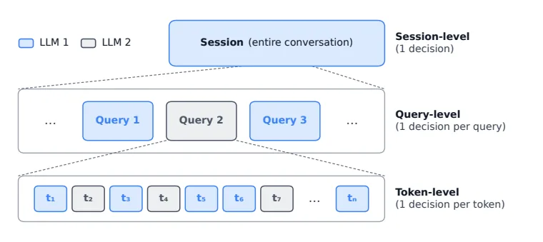
- Session/query-level: The entire request (or conversation turn) is handled by a single model. It is well compatible with existing serving stacks, but only a few discrete points on the Pareto frontier can be selected (source: §1, §2).
- Token-level: A model is selected for each token or short span. Multiple models cooperate within a single response (source: §2).
The benefits of token-level routing fall into two categories. On the efficiency side, it can exploit difficulty variation within a single query; on the quality side, models with complementary expertise can cooperate within one response to surpass the quality of a single LLM (source: §1). It also lets the cost–quality tradeoff be controlled smoothly rather than at a few discrete points.
Three Critical Obstacles
However, existing serving systems stand on the single-LLM assumption that “all active requests are synchronized at every decoding step.” Token-level routing changes the target model at every step, breaking this assumption and causing the following three problems (source: §1, §4).
- Step desynchronization: The per-step latency varies greatly across models. When requests are bundled into a single batch and synchronized, every step must wait for the slowest model, leaving fast models idle.
- Batch admission delay: Token-level routing causes frequent model switches, so a routed request easily arrives while the target model is still processing the previous batch. The request must then wait until it is admitted into the next batch, creating bubbles and batch fragmentation.
- Implementation complexity: Existing systems do not even provide a programming interface for per-step routing decisions. Implementing token-level routing internally requires extensive modification of a large codebase and delicate coordination with features like continuous batching and prefix caching.
The research gap this paper identifies is that, because the standard serving stack in effect never provided “a means to think about routing separately from serving optimization,” the theoretical benefits proven in algorithmic research could not be converted into real speed.
New Approach: TokenRouter
TokenRouter is an efficient and developer-friendly serving system for token-level routing inference. The central design principle is summarized in one sentence (source: §Abstract, §1):
Request-centric programming, model-centric execution
Developers only need to describe “how a single request flows among cooperating LLMs,” and the runtime handles efficient serving through asynchronous, model-centric subservers. This separation hides the complexity of routing serving from developers and lets the runtime fully optimize cross-model execution and batch scheduling. Only a single server interface is exposed externally, so it can be used as a drop-in replacement for existing single-LLM servers (vLLM/SGLang) (source: §4).
1) Request-Centric Programming: route–send–receive
Token-level routing algorithms differ in policy but share a common execution lifecycle (source: §2, §3):
$$ \textbf{receive} \rightarrow \text{decode} \rightarrow \textbf{route} \rightarrow \textbf{send} \rightarrow \text{peer receive} \rightarrow \text{peer decode} \rightarrow \cdots $$TokenRouter’s interface abstracts this lifecycle into three functions (source: §3).
- route(
result): Called after each decoding step; examines forward results such as hidden states, next-token logits, and sampled tokens to determine the destination index of each request in the batch. Destination0means continued local decoding, and a nonzero value means delegation to that peer model. - send(
req): Called when route delegates a request, producing a customPeerReqmessage. It contains the request ID, the token suffix the peer has not yet seen, the request’s active/finished status, and algorithm-specific fields. It attaches a location anchor calledreq.locso the peer can determine the minimal suffix to send back. - receive(
peer_req): Called when a peer’sPeerReqarrives; converts it into the local request format. The default behavior is to commit all transmitted tokens, and it need only be overridden when the handoff semantics differ across algorithms.
These three functions can express all five representative algorithms (source: §3, Tab. methods):
| Algorithm | #Models | Model $i$ | Model $j$ |
|---|---|---|---|
| CITER | 2 | low-confidence token | after 1 token |
| R2R | 2 | prediction-divergence token | after 1 token |
| R-Stitch | 2 | high-entropy token | low-entropy token |
| Co-LLM | 2 | high-deferral token | after 1 token |
| ME | $\geq$2 | after every token, according to ensemble weights |
In this way, the algorithms use different routing signals (confidence, entropy, divergence prediction, ensemble weights), but all are expressed with compact route/send functions, and the default receive suffices.
2) Asynchronous Execution: A Decoupled Tri-Loop + Handoff-Resume
To resolve step desynchronization, TokenRouter adds a decoupled inter-model loop to the standard structure of single-LLM serving (source: §4). A standard server has two asynchronous loops—a client-server loop (purple) handling request admission and response streaming, and a decoding loop (blue) handling request scheduling and model execution. TokenRouter adds a third inter-model loop (black) that exchanges peer requests between subservers.
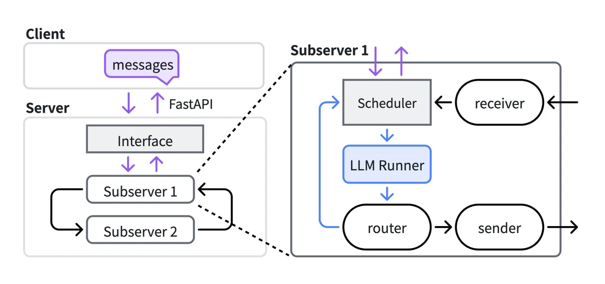
Thanks to this third loop, a routed request can leave the local batch and then resume once the peer request returns. While the request is being processed at the peer model, the remaining local requests continue at the speed of the local decoding loop. That is, each subserver proceeds at its own pace, and routed requests move between models asynchronously (source: §4).
An important optimization here is the handoff-resume mechanism. Naively, a returning request would be treated as a “new request,” requiring prefix matching and KV-cache reallocation to be redone. TokenRouter introduces a pending state between the two standard states running/finished. A pending request is skipped by the scheduler (like finished) but its serving state is fully preserved (like running). On resume it transitions to running or finished according to the peer output, and is re-admitted into the batch with the new token attached, “as if it had never left.” This skips prefix matching and KV reallocation, reducing inter-model switching to the level of “appending one token” (source: §4).
3) Delayed Batching Scheduler
Although asynchronous execution removes synchronization between subservers, each subserver still needs a scheduling policy to handle the “sparse and irregular arrival of routed tokens.” Batch admission delay is defined as the waiting time from when a request arrives at a subserver to when its execution begins (source: §4).
The core idea is to wait for a short, controlled interval to gather requests headed to the same model and execute them together. The scheduler buffers incoming requests and only executes a batch when the buffer size reaches a threshold $B$. Early-arriving requests wait longer, but late-arriving requests wait much less, so the average batch admission delay across the workload decreases.
The figure below contrasts four scheduling strategies.
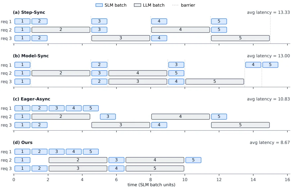
How to choose $B$ is the key here. If $B$ is too small, the batch admission delay grows; if too large, requests get stuck in the queue and the SLM starves with nothing to do. TokenRouter resolves this tradeoff mathematically (source: §4, Appx. math_model). This is covered in detail in “How It Works” below.
How It Works: A Walkthrough with Concrete Examples
Example 1 — Expressing R-Stitch with route–send–receive
Consider R-Stitch, in which a small model (SLM) and a large model (LLM) cooperate. The idea is that “tokens the SLM is uncertain about (high-entropy) are delegated to the LLM, and certain tokens are generated by the SLM itself.” On the LLM side, conversely, low-entropy tokens are sent back to the SLM.
The SLM-side implementation takes just three functions (source: §3, Fig. rstitch):
class RStitchSLM(BaseRouter):
    # self.tau (threshold) and self.peer_idx (LLM subserver index) come from config.

    def route(self, result):
        # Delegate high-entropy tokens to the LLM and keep the rest local.
        probs = result.logits_output.next_token_logits.softmax(dim=-1)
        entropy = -(probs * probs.log()).sum(-1) / math.log(probs.shape[-1])
        destination = torch.zeros_like(entropy, dtype=torch.long)
        destination[entropy > self.tau] = self.peer_idx
        return destination.cpu()

    def send(self, req) -> PeerReq:
        # Discard the just-decoded uncertain token so the LLM regenerates from that position.
        token_ids = req.origin_input_ids + req.output_ids[:-1]
        peer_anchor = req.peer_locs[self.peer_idx] or 0
        return PeerReq(rid=req.rid, token_ids=token_ids[peer_anchor:],
                       loc=len(token_ids), finished=req.finished(), ...)

# receive falls back to the default (accepting all transmitted tokens).Let’s go through step by step what each function does.
- route: Takes the softmax of the forward result’s next-token logits to obtain a probability distribution, and computes the normalized entropy. It sets the destination of tokens exceeding the threshold
tau($0.03$ in R-Stitch) topeer_idx, and the rest to0(local). - send: On delegation, it transmits only the suffix excluding “the uncertain token just sampled” (
output_ids[:-1]), so that the LLM regenerates from that position. Viapeer_anchor, it trims the part the peer already knows and sends only the minimal suffix. - receive: Accepts all tokens returned by the LLM (the default behavior).
The key insight is that developers need not worry at all about batches, scheduling, or asynchronous execution. They simply fill in the three functions along the trajectory of a request flowing SLM→LLM→SLM. On the LLM side, the only difference is changing > in route to <= (source: §3).
Example 2 — How Delayed Batching Reduces Batch Fragmentation
Suppose there are two models (SLM and LLM), the LLM’s delayed batching threshold is $B=2$, and the SLM’s is $B=1$ (immediate execution) (source: §4, Fig. schedule).
- A token of request 1 arrives at the LLM. Only one is in the buffer, so no batch is executed.
- A token of request 2 arrives. The buffer reaches $B=2$, so the two requests are bundled into one batch and executed.
- When the LLM forward finishes, both tokens are committed together, and the requests return to the SLM and continue.
With an eager approach, the LLM would be invoked immediately for request 1’s token, and request 2’s token arriving during that execution would have to wait until the next batch. Delayed batching amortizes the LLM’s fixed overhead (kernel launch, memory access, etc.) over a wider batch, so the average admission delay drops and throughput rises.
Example 3 — The Mathematical Model for Finding the Optimal Threshold $B^*$
TokenRouter determines the throughput-optimal value $B^*$ of the delayed batching threshold analytically. It models the routing process as a discrete-time Markov chain (DTMC) (source: §4, Appx. math_model).
The system state is expressed by each model’s (waiting queue $k_i$, running batch $b_i$, remaining execution time $r_i$). A request that completes one step at model $i$ is routed to model $j$ with probability $p_{ij}$ and commits $c_{ij}$ output tokens. The model defines the routing transition matrix $\mathbf{P}$ and the token commit matrix $\mathbf{C}$.
For example, in the case of R2R (two models, $M=2$):
$$ \mathbf{P} = \begin{bmatrix} 1-p & p\\ 1 & 0 \end{bmatrix}, \qquad \mathbf{C} = \begin{bmatrix} 1 & 0\\ 1 & 0 \end{bmatrix} $$Here $p$ is the probability that the SLM, after generating one token, hands it to the LLM. The structure is that either the SLM commits directly ($1-p$), or the LLM commits the corrected token (the second row of $\mathbf{C}$).
Observing the system at batch completion times yields a finite-state DTMC. Solving for the stationary distribution $\boldsymbol{\pi}_{\mathbf{B}}$, the steady-state throughput $T(\mathbf{B})$ is “expected number of committed tokens ÷ expected holding time”:
$$ T(\mathbf{B})
\frac{ \sum_{\mathbf{s}\in\mathcal{R}{\mathbf{B}}} \pi{\mathbf{B}}(\mathbf{s}) \sum_{i\in\mathcal{A}(\mathbf{s})}\sum_{j=0}^{M-1} b_i, c_{ij}, p_{ij} }{ \sum_{\mathbf{s}\in\mathcal{R}{\mathbf{B}}} \pi{\mathbf{B}}(\mathbf{s}),\tau(\mathbf{s}) } $$
Finally, under a feasibility condition that prevents deadlock (a state in which no model has enough requests to start a batch), it finds the $\mathbf{B}^\star$ that maximizes throughput:
$$ \sum_{i=0}^{M-1}(B_i - 1) < N $$The authors compared this model against measurements for R2R. With SLM step latency $L_0 = 6.0\,\mathrm{ms}$, LLM step latency $L_1 = 27.9\,\mathrm{ms}$, time quantum $\delta = 0.1\,\mathrm{ms}$, and $p = 0.35$, the optimal threshold predicted by the model matched the measured optimal threshold at all concurrency levels (source: Appx. math_model).
To summarize the roles of these three mechanisms — route–send–receive delivers expressiveness, the asynchronous tri-loop removes desynchronization, and delayed batching prevents batch fragmentation. On top of these, routing-specific engineering optimizations such as CUDA graph capture, in-process routers, and automatic KV-cache allocation are added (source: Appx. opt).
Performance Validation: Main Results
Experimental Setup
- Five algorithms: CITER, R2R, R-Stitch, Co-LLM, ME. The first four route between Qwen3-0.6B ↔ Qwen3-32B, and ME routes among the three models Qwen3-0.6B/8B/32B (source: §5).
- Hardware: An 8×A100-80G server. Two-model algorithms use 1 GPU for the SLM and 2 GPUs for the LLM (tensor parallel), shared via CUDA MPS (source: §5).
- Baselines: The official algorithm implementations (Official Code) and an SGLang-based Std. Serving built for a fair comparison (source: §5).
- Three workloads: Low-effort reasoning (AIME2024, input ~100 tokens / output up to 2048), High-effort reasoning (output up to 8192), and Agentic (SWE-Smith, input ~8192 / output up to 1024) (source: §5).
Throughput: Up to 64×
In all 15 algorithm-workload combinations, TokenRouter recorded 2.01–64.15× the throughput of the stronger baseline, and reduced end-to-end latency by 2.03–63.64× versus Std. Serving (source: §5, Fig. throughput_bs4). The gains are especially large for Co-LLM and CITER. This is because the official implementations often lacked even continuous batching, and Std. Serving lacks handoff-resume and so cannot preserve the serving state of routed requests.
Let’s look at the table comparing under the original algorithm settings (concurrency 4) (source: Tab. e2e_latency_bs4):
| Algorithm | Implementation | Throughput (token/s) | TTFT (s) | Latency (s) | |—|—:|—:|—:| | R2R | LLM-only | 145.30 | 0.13 | 411.98 | | | Official Code | 89.62 | 0.11 | 751.15 | | | TokenRouter | 244.56 | 0.11 | 270.19 | | CITER | LLM-only | 123.72 | 0.083 | 2.68 | | | Official Code | 17.16 | 0.036 | 7.64 | | | TokenRouter | 149.31 | 0.036 | 0.48 | | Co-LLM | LLM-only | 134.79 | 0.069 | 13.39 | | | Official Code | 3.46 | 1.14 | 247.61 | | | TokenRouter | 76.02 | 0.067 | 11.46 | | R-Stitch | LLM-only | 150.41 | 0.15 | 360.76 | | | Official Code | N/A | N/A | N/A | | | TokenRouter | 140.58 | 0.067 | 151.30 |
A notable point: CITER raises throughput to 149.31 token/s while cutting latency to 0.48 s, making it far faster than LLM-only (2.68 s). That is, routing enables serving that maintains quality while being faster than a single large model.
Where Do the Performance Gains Come From?
Decomposing the gains at concurrency 8 (source: §5, Tab. gain_source):
| Configuration | $N=8$ throughput (token/s) |
|---|---|
| TokenRouter (full) | 372.48 |
| − delayed batching | 296.86 |
| − asynchronous execution | 230.79 |
| − router CUDA graph | 228.10 |
| − LLM CUDA graph | 164.08 |
| − SLM CUDA graph (≈ R2R official) | 132.78 |
| R2R official code | 134.89 |
Engineering optimizations alone (extending CUDA graph capture) raise the baseline from 132.78 → 230.79 token/s (about 1.71×), and layering on asynchronous execution and delayed batching reaches 372.48 token/s (2.76× total) (source: §1, §5).
The clue to understanding the gap with Std. Serving lies in the latency breakdown. On the SLM side, for the per-step latency (average over the last 128 steps of generating 2048 tokens) (source: Appx., Tab. slm_latency_breakdown):
| Operation | Latency (ms) | Ratio |
|---|---|---|
| Prefix matching | 7.78 | 20.94% |
| Update radix cache | 12.12 | 32.62% |
| Locking cache nodes | 6.49 | 17.47% |
| Releasing locks | 5.13 | 13.81% |
| SLM inference | 1.56 | 4.20% |
| Others | 4.08 | 10.98% |
Strikingly, actual SLM inference is only 4.20%, and the rest is all overhead from the single-model assumption of “treating a returning request as a new request.” TokenRouter preserves the request-level KV-cache state across model switches and resumes immediately when the peer result arrives, eliminating most of this overhead (source: Appx.).
Throughput–Speed Tradeoff
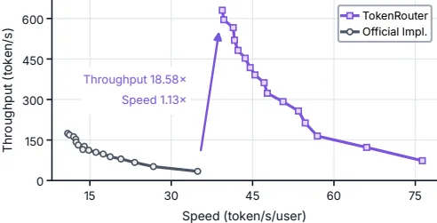
Raising concurrency from 1 to 16 increases TokenRouter’s throughput by 8.61× while maintaining 51.7% of single-user speed. In contrast, official R2R increases by only 5.14× while maintaining 31.3%. In particular, at concurrency 16, TokenRouter delivers 18.58× the throughput of R2R at concurrency 1 while being 1.13× faster per user — that is, throughput is overwhelmingly higher even under a stricter speed SLO (source: §5).
Generalization Validation
- Varying model pairs: Across all four pairs 0.6B-8B, 0.6B-32B, 1.7B-8B, and 4B-8B, 1.99–3.21× over official R2R (source: §5, Tab. r2r_tokenrouter_gain_app).
- Scaling output length: Going from low-effort (up to 2048) to high-effort (up to 8192), TokenRouter’s throughput is maintained, whereas Std. Serving loses 58.1–85.2% of its throughput (source: §5).
- Distributed deployment: Even in a cross-node deployment with two nodes connected via RoCE (3.7 GB/s), throughput is similar to a single node (1.93–32.81× over official) (source: Appx.).
- Pareto frontier: TokenRouter pushes token-level routing to a new Pareto frontier, making it competitive with coarse-grained query routing on top of SOTA frameworks like SGLang (source: §5).
Our Perspective: Strengths, Limitations, and Why This Research Matters
Strengths
- Clean problem formulation and clear separation of contributions. The structure is convincing: it names the three obstacles (desynchronization, admission delay, implementation complexity) and maps each one-to-one to a mechanism that solves it (asynchronous tri-loop, delayed batching, route-send-receive).
- Separation of “expressiveness” and “execution.” The abstraction that developers need only draw the request trajectory is simple yet powerful. The fact that five algorithms run on the same runtime proves its generality (source: §3, §5).
- Theory–measurement agreement. Deriving the delayed batching threshold via a DTMC and showing that the predicted optimum matches the measured optimum is a rare strength in an engineering paper (source: Appx.).
- Honest baselines. Where no official implementation existed, rather than just leaving it as “N/A,” they built an SGLang-based Std. Serving themselves for a fair comparison. The overhead breakdown table (Tab. slm_latency_breakdown) transparently shows the source of the gains.
Limitations and Caveats
- Assumptions of the mathematical model. As the authors themselves acknowledge, the model assumes that the number of tokens between two consecutive sends follows a geometric distribution. This holds for most algorithms, but corner cases that violate it remain unresolved (source: §6).
- Scope of hardware and scale. The evaluation centers on a single 8×A100-80G server, and the in-depth analysis of ME’s multi-model (≥3) scenario is relatively thin. Scalability on newer GPU generations or inference-specialized hardware (H100/MI300, etc.) has not been validated.
- The quality of the routing algorithm itself is not under test. This paper addresses “how fast a given routing algorithm can be served.” The accuracy and quality preservation of the router are the concern of each original paper. The throughput–accuracy tradeoff is only partially addressed.
- Subtleties of comparison created by CUDA MPS-based GPU sharing. A setting in which two models share a GPU requires interpretation regarding resource fairness. The paper is conscious of this and covers non-overlap batching (+6.43%) and parallel strategies in the appendix (source: Appx.).
Why It Matters
Token-level routing is a practically very attractive cost-saving strategy of “a small model + selective calls to a large model.” Although R2R showed figures like “only 5% of tokens to 32B,” the stumbling block was that actual serving speed did not live up to expectations. TokenRouter provides the system-layer infrastructure that bridges that gap. It is significant in that it is a foundation on which future token-level routing algorithm research can move from “theoretical benefits” to “measured speed.”
What’s Next?: The Road Ahead
Focusing on the problems the authors left open, reasonable next steps are as follows.
- Generalizing the mathematical model. Relax the geometric distribution assumption and extend to a model that can handle state-dependent, time-varying routing probabilities and non-stationary arrivals. The commented-out general model in the appendix sketches a direction for this.
- In-depth optimization for three or more models (ME). Currently ME is only validated at the feature level; there is ample room in the joint optimization of multi-model handoff costs and delayed batching thresholds.
- Diverse hardware and serving backends. Beyond the SGLang-based implementation, integration with vLLM, TensorRT-LLM, etc., and reproduction on a wider range of GPU generations and inference chips.
- Co-design of routing policy and scheduler. The delayed batching threshold $B^*$ depends on the routing probability $p$. Jointly learning/searching the routing policy and the serving scheduler could be interesting follow-up research.
- Consistency with quality metrics. Systematically validating the throughput–accuracy Pareto frontier across a wider range of benchmarks to confirm that system optimization does not compromise routing quality.
Tables from the paper
Tables converted mechanically from the arXiv e-print LaTeX source. The numbers are the paper’s own and did not pass through a model.
Table 1. Routing behavior of the evaluated token-level routing algorithms. Each entry under Model $i$ or Model $j$ specifies the condition under which that model routes generation to another model.
| Algorithm | #Models | Model $i$ | Model $j$ |
|---|---|---|---|
| CITER | 2 | low-confidence token | after one token |
| R2R | 2 | predicted-divergent token | after one token |
| R-Stitch | 2 | high-entropy token | low-entropy token |
| Co-LLM | 2 | high-deferral token | after one token |
| ME | $\geq$2 | after every token, according to ensemble weights |
Table 2. TTFT, throughput, and end-to-end latency at concurrency 4, comparing across serving systems under original settings.
| Algorithm | Implementation | Throughput/(token/s) | TTFT/s | Latency/s |
|---|---|---|---|---|
| R2R | LLM-only | 145.30 | 0.13 | 411.98 |
| Official Code | 89.62 | 0.11 | 751.15 | |
| TokenRouter | 244.56 | 0.11 | 270.19 | |
| CITER | LLM-only | 123.72 | 0.083 | 2.68 |
| Official Code | 17.16 | 0.036 | 7.64 | |
| TokenRouter | 149.31 | 0.036 | 0.48 | |
| Co-LLM | LLM-only | 134.79 | 0.069 | 13.39 |
| Official Code | 3.46 | 1.14 | 247.61 | |
| TokenRouter | 76.02 | 0.067 | 11.46 | |
| R-Stitch | LLM-only | 150.41 | 0.15 | 360.76 |
| Official Code | N/A | N/A | N/A | |
| TokenRouter | 140.58 | 0.067 | 151.30 |
Table 3. Model pairs and benchmarks used by different token-level routing algorithms.
| System | Model Pair | Benchmark |
|---|---|---|
| R2R | DeepSeek-R1-Distill-Qwen-1.5B / 32B | AIME |
| CITER | Qwen2-1.5B / 72B | CommonsenseQA |
| Co-LLM | LLaMA2-7B (tuned) / 70B | GSM8K |
| R-Stitch | L1-1.5B-Short / QwQ-32B | AIME |
Table 4. TTFT, throughput, and end-to-end latency at concurrency 1, comparing across serving systems under original settings.
| Algorithm | Implementation | Throughput/(token/s) | TTFT/s | Latency/s |
|---|---|---|---|---|
| R2R | LLM-only | 40.17 | 0.074 | 388.12 |
| Official Code | 54.77 | 0.12 | 330.69 | |
| TokenRouter | 105.81 | 0.11 | 144.10 | |
| CITER | LLM-only | 34.40 | 0.055 | 2.42 |
| Official Code | 14.26 | 0.031 | 2.41 | |
| TokenRouter | 50.63 | 0.031 | 0.36 | |
| Co-LLM | LLM-only | 36.06 | 0.049 | 12.66 |
| Official Code | 2.80 | 0.34 | 76.68 | |
| TokenRouter | 28.57 | 0.068 | 7.60 | |
| R-Stitch | LLM-only | 40.82 | 0.072 | 341.84 |
| Official Code | N/A | N/A | N/A | |
| TokenRouter | 55.78 | 0.102 | 119.29 |
Table 5. Ablation study of different optimization components. Throughput is reported in token/s.
| Method | $N=8$ | $N=4$ | $N=1$ |
|---|---|---|---|
| TokenRouter | 372.48 | 210.61 | 73.02 |
| - Delayed batching | 296.86 | 161.26 | 73.02 |
| - Async execution | 230.79 | 143.88 | 73.02 |
| - Router CUDA graph | 228.10 | 142.33 | 72.62 |
| - LLM CUDA graph | 164.08 | 95.55 | 51.22 |
| - SLM CUDA graph ($\approx$ R2R) | 132.78 | 75.54 | 34.20 |
| R2R official code | 134.89 | 73.27 | 36.17 |
Table 6. Throughput across parallel strategies. Throughput is reported in token/s.
| Total | #SLM | #LLM | Overlap | $N{=}1$ | $N{=}4$ |
|---|---|---|---|---|---|
| 2 | 1 | 1 | $\times$ | 50.37 | 160.74 |
| 1 | 2 | $\checkmark$ | 70.83 | 197.40 | |
| 2 | 2 | $\checkmark$ | 71.41 | 198.13 | |
| 8 | 4 | 4 | $\times$ | 93.23 | 284.62 |
| 1 | 8 | $\checkmark$ | 109.67 | 296.34 | |
| 2 | 8 | $\checkmark$ | 106.02 | 289.08 | |
| 4 | 8 | $\checkmark$ | 110.02 | 297.63 | |
| 8 | 8 | $\checkmark$ | 105.59 | 288.35 |
Table 7. Throughput (token/s) comparison across routing strategies under different concurrency and overlap settings.
| Setup $N$ | Setup Deployment | Routing Algorithm R2R | Routing Algorithm R-Stitch | Routing Algorithm Co-LLM | Routing Algorithm CITER |
|---|---|---|---|---|---|
| 1 | Overlapping | 73.27 | 43.06 | 47.46 | 102.29 |
| Non-overlapping | 74.90 | 47.53 | 48.25 | 108.65 | |
| 4 | Overlapping | 205.05 | 108.42 | 165.96 | 281.27 |
| Non-overlapping | 228.94 | 116.14 | 170.20 | 308.36 |
Table 8. Throughput comparison across single-node and multi-node settings.
| Setup $N$ | Setup Deployment | Routing Algorithm R-Stitch | Routing Algorithm R2R | Routing Algorithm CITER |
|---|---|---|---|---|
| 1 | Single-node | 47.53 | 74.90 | 108.65 |
| Multi-node | 46.19 | 69.92 | 93.99 | |
| 4 | Single-node | 116.14 | 228.94 | 308.36 |
| Multi-node | 104.20 | 202.43 | 277.56 |
Figures in this post are taken from the original arXiv:2610.12242 (CC BY 4.0). Only size and format were changed.
Comments