Rethinking Loop Models at the Fixed Point — Four Shortcuts That Erase the Cost of Recursion
TL;DR
In looped language models, the state converges to a fixed point $z^\star = F_\theta(z^\star; x)$ as the recursion depth grows, and near the fixed point the “endpoint” can stand in for the entire trajectory. This paper uses that one property to reduce four different costs at once across pretraining, serving, and RL: (1) training backpropagates only through the last $b$ recursions (truncated BPTT), (2) decoding caches only the last KV bank for each token (terminal KV sharing, a $3\times$ cut in cache), (3) prefill is distilled into a lightweight student that predicts the fixed point directly, giving up to a $1.79\times$ speedup, and (4) RL reuses gradients from stored rollout states to make updates $2\times$ faster. It also improves the two devices that actually produce this fixed point — the depth prior and input injection — as a “learned prior” and “orthogonal injection (OrthoInj)” respectively, lowering perplexity across the whole range from 100M to 1.6B parameters (source: §1).
Core Idea
The claim of this work can be summarized in one sentence: “If you just train properly to create a fixed point, you can remove most of the ‘cost proportional to depth’ that loop models pay.”
Concretely, it splits into two branches.
- Four shortcuts the fixed point provides (source: §3): The fact that the endpoint can stand in for the trajectory translates directly into cost savings at each stage — training, inference, and post-training — as shown through theory (a Lemma) and experiments.
- Improving the two devices that create the fixed point (source: §4): What actually forms the fixed point are the depth prior (at which depth supervision is received) and input injection (how the input persists at the fixed point); existing options (Huginn’s PLN prior, Parcae’s injection) each have limitations, so this work replaces them with a learned prior and orthogonal injection.
Background: The Problem They Solved
In Loop Models, “Depth” Is Cost
Looped language models apply the same layer block repeatedly (source: §2). Starting with the Universal Transformer, recent work such as Huginn and Ouro uses them for test-time compute scaling and latent reasoning. The essential cost of this structure, however, arises “on every iteration” (source: §1):
- Training: The full recursion must be stored and backpropagated, so activation memory scales with depth.
- Decoding: Each recursion uses its own KV, so the KV cache grows with depth.
- Prefill: Every recursion must be run for each prompt token.
- RL: Every rollout must re-run the recursion for scoring.
“Should We Learn a Fixed Point?” Is Still Unresolved
The field has split into two camps (source: §1). One gives up on the fixed point and fixes the number of loops to a small value (Loopie, Smelt, Ouro). The other deliberately forms a fixed point and loops deeply (the DEQ, STaR, EQR line). This paper pushes the latter camp’s position that the fixed point is the key to cost reduction.
The core observation is empirical. Terminal KV sharing (reusing only the last KV) barely degrades GSM8K performance in Huginn, but collapses at four loops in Ouro. This difference aligns exactly with whether the state converges: Huginn’s state approaches a fixed point, while Ouro’s does not (source: §1, §2).
What Is a Fixed Point
Let the state after $r$ recursions for input $x=(x_1,\dots,x_N)$ be $z^r=(\mathbf{H}^r, C^r)$. Here $\mathbf{H}^r$ is the hidden state and $C^r$ is the KV bank recorded at the $r$-th update. The shared update map $F_\theta$ defines $z^{r+1}=F_\theta(z^r;x)$, and if $F_\theta(z^\star;x)=z^\star$ holds, then $z^\star$ is the fixed point (source: §2).
Convergence is measured by the per-token relative change $\rho_{r,t}=\lVert h_t^r-h_t^{r-1}\rVert_2/(\lVert h_t^{r-1}\rVert_2+\epsilon)$ ($\epsilon=10^{-8}$). An important finding: convergence is heterogeneous. Even within the same sequence, tokens converge at different depths, the order is not causal, and the Spearman correlation between convergence depth and position is a weak $0.14$ (source: §2). This heterogeneity is exactly why “which depth receives supervision” matters.
Experimental Model Configuration
The experiments are run on a dense Llama-block loop model based on Huginn (source: §5.1, Tab. 1). The layout is 1+2×R+1: one prelude block → a 2-block recursion core repeated $R$ times → one coda block. That is, $R=5$ recursions give a logical depth of $12$ blocks. There are three scales: Small (100M, 21.5B tokens), Medium (400M, 85.9B), and Large (1.6B, 343.6B). They use the Jais64k tokenizer, the TxT360 multilingual mixture, a sequence length of 8,192, and AdamW with a WSD schedule.
New Approach: Learned Depth Prior + Orthogonal Input Injection (OrthoInj)
To actually get the benefits of the fixed point, training must form it. The two devices governing its formation are the depth prior and input injection, and this paper improves both.
1) Learned Depth Prior — Learning “Which Depth to Supervise”
The sampled training depth determines “how converged the state is when supervision arrives,” and therefore how well it tolerates terminal KV sharing (source: §4.1).
- Fixed-depth training: Concentrating supervision on a single depth gives the best predictions at that depth, but it breaks KV sharing. In the 1.6B model, sharing halves GSM8K from $50.6 \to 21.2$ (source: §1).
- Huginn’s PLN prior: Spreading depth over a shifted Poisson–lognormal distribution supports sharing, but dilutes supervision at the target depth below the level sharing requires.
The authors therefore learn the depth prior. Instead of PLN, they place a categorical distribution $p_\phi=\operatorname{softmax}(\phi)$ over the depth set $\mathcal R=\{1,\dots,R_{\max}\}$ and update the logits $\phi$ from prediction feedback (source: §4.1, Alg. 1):
$$ \mathcal J_{\mathrm{prior}}(\phi) = -\widehat{\mathbb E}{n}\bigl[\operatorname{sg}(A_n)\log p\phi(r)\bigr]
- \lambda_H, H(p_\phi)
- \lambda_m\bigl(\mathbb E_{p_\phi}[R] - \bar R\bigr)^2 $$
The role of the three terms is clear.
- Prediction quality: For each microbatch, sample a depth $r$, map the next-token CE $\ell$ at that depth to a reward $u=\exp(-\ell)$ (inverse perplexity), center it with an EMA baseline, rescale it PopArt-style, and multiply by the advantage $A_n$. Depths that predict well get higher probability.
- Entropy regularization $H(p_\phi)=-\sum_r p_\phi(r)\log p_\phi(r)$: With feedback alone, supervision concentrates on a narrow depth and fixed-point formation weakens. Increasing $\lambda_H$ spreads the allocation toward deeper depths (the region where the settled prefix context supports sharing). In other words, $\lambda_H$ is the knob that trades off performance against memory efficiency.
- Budget control: Keeps the expected depth from drifting away from the target $\bar R$. Since the prior is used only in training, this term pins the forward-pass compute to $\bar R$.
Unlike RL-Halting and Ouro’s “state-dependent exit distribution,” this prior is unconditional, so (1) it can start from a predefined prior (PLN), (2) it saves compute by running the forward pass only to the sampled depth, and (3) it does not decide the stopping point at inference, allowing the entropy term to deliberately increase KV sharing (source: §6, Appx.).
2) Orthogonal Input Injection (OrthoInj) — Making “the Input Remain Intact at the Fixed Point”
Input injection adds the embedding to every recursion so that the fixed point is conditioned on the input. The general additive form is $\zeta_t^r = M h_t^r + q_t$ (source: §4.2). Here $M$ controls the state carryover and $q_t$ is the injection vector. Parcae uses a diagonal carryover $M=\Lambda=\operatorname{diag}(\exp(-\Delta\odot\alpha))$ (entries of $\Lambda$ in $(0,1)$, $\lVert\Lambda\rVert_2<1$).
The problem is that the carryover $\Lambda h_t^r$ can have a component along the injection vector $q_t$. Depending on the sign of this component, it amplifies or cancels the input. Measured on Parcae-Decay, the cosine between the carryover and $q_t$ reaches $0.81/0.87/0.91$ for S/M/L, so the input enters the core at $2.2\times/2.8\times/3.4\times$ its injected magnitude (source: Appx.). OrthoInj projects out this component:
$$ \zeta_t^r = Q_{q_t}\Lambda h_t^r + q_t, \qquad Q_{q_t} = I - \frac{q_t q_t^{\top}}{\lVert q_t\rVert_2^2 + \epsilon} $$$Q_{q_t}$ is the projection that removes the component along $q_t$. As a result, at every recursion (including the fixed point), the component of $\zeta_t^r$ along $q_t$ becomes exactly $q_t$, and only the orthogonal component evolves freely. Since $\lVert Q_{q_t}\rVert_2\le1$, the contraction property of the carryover ($\lVert Q_{q_t}\Lambda\rVert_2\le\lVert\Lambda\rVert_2<1$) is also preserved.
How It Works: A Concrete Example
Toy Example: The Fixed Point of a Contraction Map
Let us look at the idea with a very simple one-dimensional map. If the state update is $z^{r+1} = 0.5\, z^r + 3$ and $z^0=0$, then the fixed point is $z^\star = 0.5 z^\star + 3 \Rightarrow z^\star = 6$. Running the iteration gives:
| $r$ | 0 | 1 | 2 | 3 | 4 | 5 | … |
|---|---|---|---|---|---|---|---|
| $z^r$ | 0 | 3 | 4.5 | 5.25 | 5.625 | 5.8125 | $\to 6$ |
Because the contraction factor $a=0.5<1$, the difference between adjacent states shrinks geometrically: $|z^{r+1}-z^r|=0.5^r \cdot 3$. That is, near the fixed point the state barely changes no matter how much more you iterate. This is the principle shared by every shortcut in this paper: you can use the endpoint $z^\star$ instead of the trajectory.
The same story holds from the gradient perspective. Differentiating the loss with respect to $z^\star$ gives $\mathrm dz^\star/\mathrm d b = 1/(1-a)=2$, which is the sum of the Neumann series $1+a+a^2+\cdots$. In practice, this infinite sum can be cut off at $b$ terms (truncation), and the error $a^b$ shrinks geometrically in $b$ (source: §3.1).
How This Principle Becomes Four Shortcuts
Training — truncated BPTT: Instead of backpropagating through all $R$ recursions, backpropagating through only the last $b$ suffices. Near the fixed point the visited states converge to $z^\star$, so the TBPTT gradient converges to a truncated Neumann estimate of the equilibrium gradient (implicit gradient) (source: §3.1, eq. 1). The surprising part is that truncation itself forms the fixed point. At a fixed depth of $R=5$, full BPTT raises perplexity by more than $25\%$ when extrapolated to $R=64$ and by $21\%$ under terminal KV sharing, whereas TBPTT backpropagating only the last 2 ($b=2$) raises them by no more than $2\%$ and $3\%$, respectively (source: §3.1).
Decoding — terminal KV sharing: Keep only the last KV bank of each prefix token, and let all recursions of subsequent tokens read from it. At $R=5$, keeping only $4$ of $12$ banks cuts the cache by $3\times$, and the perplexity increase is no more than $0.85\%$ (source: §3.2). Theoretically, the Lemma supports this: if the prefix KV converges to $C^\star_{
Prefill — distillation: Since decoding reads only the last bank, prefill need not “reproduce all KV of every recursion” — it only needs to predict the endpoint. A lightweight student $S_\psi$ predicts $\widehat z = S_\psi(e)\approx z_\theta^R(x)$ from the prelude output $e$, and the teacher applies one recursion to $\widehat z$ to produce all KV banks. The loss is a normalized hidden-state regression plus a next-token KL:
$$ \mathcal L_{\mathrm{distill}}(\psi) = \mathbb E_x\left[ \frac{\lVert\widehat z - z_\theta^R(x)\rVert_F^2}{N d \sigma_T^2}
- \frac{1}{N}\sum_{t=1}^{N}\operatorname{KL}\bigl(p_t ,\Vert, \widehat p_t\bigr) \right] $$
Since the student is initialized from the teacher’s recursion core, before training it roughly outputs “the state after 1 recursion,” and the loss pushes this toward the depth-$R$ endpoint (source: §3.2, §5.5).
- RL — reusing rollout states: RL typically runs the forward pass twice (once for sampling, once for scoring). Near the fixed point, it computes the Neumann-$(b-1)$ gradient directly from the stored endpoint $z^R$ without re-running the recursion (source: §3.1, Alg. 2). Run the recursion block through $z^R$ only once to record its autograd graph, then iterate $v \leftarrow g + J_R^{\top} v$ for $b-1$ steps to obtain the gradient. The update cost becomes independent of $R$.
Validating Performance: Key Results
Depth Prior: Superior Across All Scales While Preserving Sharing
Four priors (fixed $R{=}5$, fixed PLN-5, learned $\lambda_H{=}0$, learned $\lambda_H{=}0.01$) were compared at an average depth of 5 (source: §5.2, Tab. 3).
- Fixed-depth training breaks KV sharing: Under sharing, GSM8K drops by more than half at M and L, and perplexity is the highest.
- The learned prior lowers validation PPL by $0.7$–$1.8\%$ versus fixed PLN-5 (using only up to $1.6\%$ extra training FLOPs), and the downstream average is higher at every scale.
- The entropy term is essential at L: Without it, GSM8K drops from $47.92 \to 36.47$ (source: §5.2).
- It dominates Untied 4 at the same physical depth and approaches Untied 12 at the same logical depth: The downstream-average lead grows from $2.2 \to 5.0 \to 8.9$ points for S→M→L. At L, the gap to Untied 12 narrows to $1.5$ points downstream average and $0.9$ points on GSM8K (source: §5.2).
In other words, at 1.6B the learned prior matches the downstream average of fixed-depth training with the full cache, using a $3\times$ smaller KV cache (source: §1, Tab. 3).
The training curves and depth distributions are shown in the figures below. Fixed depth piles up at one point, fixed PLN spreads widely, and the learned prior shifts mass between them toward “depths with good predictions.”
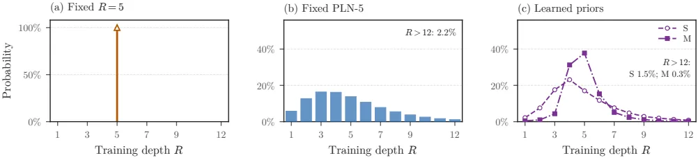
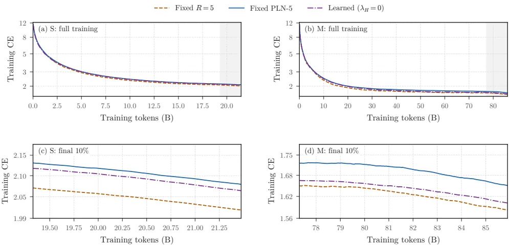
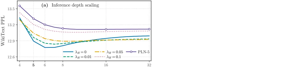
Increasing the entropy coefficient $\lambda_H$ from $0$ to $0.1$ shrinks $p_\phi(5)$ from $67.4\% \to 14.0\%$, spreading supervision toward deeper depths. As a result, the KV sharing penalty decreases monotonically (from $+0.96\% \to -0.22\%$ under sharing), and while PPL at $R=5$ rises slightly, PPL at deeper depths ($R=32$) falls — a clear trade-off between performance and memory (source: Appx.).
Orthogonal Injection: Beating the Strongest Baseline (Parcae)
OrthoInj is compared against DEQ-QKV, Huginn-Linear, and Parcae-Decay (source: §5.3, Tab. 2):
- It lowers validation PPL by $0.3$–$1.4\%$ versus the strongest baseline, Parcae-Decay.
- It has the highest downstream average at every scale, and the training loss at the end of training is also the lowest at every scale.
Each of the two switches (orthogonal projection, removing the prelude RMSNorm) lowers the loss, and their effects add up (source: Appx.).
RL: Reusing Rollout States Speeds Up Updates by $2\times$
The L learned-prior model was fine-tuned with Dr. GRPO at $R=6$ for comparison (source: §5.4, Tab. 4).
- Reuse + Neumann-4 cuts scoring and backprop time by $1.99\times$ (GSM8K) and $2.02\times$ (MBPP+).
- All four methods raise GSM8K pass@1 from $40.6\% \to 60$–$63\%$ and MBPP+ from $30.9\% \to 37$–$41\%$.
- Accuracy is within run-to-run variance of BPTT: The gradient cosine between the reuse and recompute controls is $0.997$–$0.999$, essentially identical, so the pass@1 gap ($1.6$ points on GSM8K) is at the level of run-to-run variation (source: §5.4).
- On MATH500, which is not trained in RL, transfer of $3.9$–$5.4$ points still occurs.
Distilled Prefill: Trading Latency for Accuracy
The learned-prior model was distilled into a 2-block student (using only $1/4$ of the teacher’s pretraining tokens) (source: §5.5, Tab. 5).
- Up to $1.79\times$ faster prefill on 8K prompts (S $1.55\times$, M $1.66\times$, L $1.79\times$).
- The downstream-average loss is $1.0$ (S), $2.3$ (M), and $4.5$ (L) points, growing with scale.
- At the same latency it beats stopping the teacher early: It is $0.5$–$0.9$ points higher than an $R=2$ teacher.
- Teacher initialization is the key to quality, and the KL term lifts generation performance (source: Tab. 6).
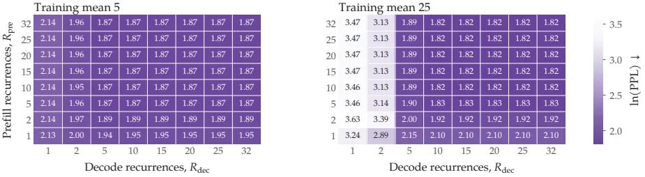
That prefill depth and decode depth can be separated (thanks to terminal sharing) is also an interesting result. As the figure below shows, the prefill gain saturates at $R_{\mathrm{pre}}=5$, whereas decode depth has a much larger effect (source: Appx.).
Our Perspective: Strengths, Limitations, and Why This Work Matters
Strengths: One Principle Cuts Through Many Problems
The greatest virtue of this paper is that it organizes four different cost problems under a single concept (the fixed point). Truncated BPTT and terminal KV sharing are shortcuts that already existed, but the authors explain “why these work” through the single framework of fixed-point convergence, and from there naturally derive two new shortcuts (distilled prefill, rollout-state reuse) (source: §1, §3). This is a rare structure in which explanatory power leads directly to new invention.
The theory–experiment alignment is also strong. The Lemma proves the limit in which “if the prefix converges, terminal sharing holds without loss,” and experiments show that the sharing penalty decreases from $0.85\%$ to $0.11\%$ as $R$ grows, matching qualitatively (source: §3.2, Appx.).
Finally, the framing that “what forms the fixed point is training design such as truncation, the depth prior, and injection” is practically very powerful. Simply reducing $b$ creates the fixed point, and the learned prior and orthogonal injection are layered on top, so each improvement connects to a clear mechanism.
Limitations: The Limits of Scale and Evidence Are Clear
The points worth criticizing are also clear.
- Scale: At most $1.6$B parameters, a single seed per configuration, and a single multilingual mixture. Whether these gains hold at 7B and above remains open (source: §7).
- Scaling of the distillation gap: The downstream loss of distilled prefill grows with scale — $1.0 \to 2.3 \to 4.5$ points for S→M→L. If this trend continues, distillation may become less attractive for large models, and the authors explicitly acknowledge this (source: §5.5, §7). Indeed, distilling an $R=25$ teacher is faster but loses more quality.
- Breadth of evaluation: Downstream tasks are centered on relatively “easy” tasks (LAMBADA, PIQA, ARC, etc.), and validation on strong reasoning benchmarks (hard coding/math) is limited.
- Assumptions: The theory (Lemma) relies on contractiveness ($\kappa<1$) and local Lipschitz conditions, but verifying or guaranteeing these in real large transformers is a separate matter.
Why It Matters
The goal of “decoupling inference cost from depth” has direct value in today’s era of LLM serving and agents. In particular, the result of cutting the cache by $3\times$ via terminal KV sharing while barely losing accuracy, and the result of speeding up RL updates by $2\times$, squarely target two practical pain points: the memory bottleneck and the post-training bottleneck. Moreover, the framework is not confined to a specific model (Huginn) but applies to recurrent structures whose states converge in general.
What’s Next?: The Road Ahead
Open questions the authors themselves leave, together with directions that follow naturally from the limitations:
- Larger scale: How the four shortcuts scale beyond 1.6B to 7B and above is the top validation task (source: §7).
- Better distillation: MoE student architectures, reallocating the distillation token budget, and better loss objectives can narrow the distillation gap. Furthermore, using the student as a standalone language model or as a drafter for speculative decoding, and connecting recurrent state refinement to flow-based language modeling, are future tasks the authors leave (source: §5.5, §3.2).
- Robustness and practical deployment: Beyond the single-seed, single-dataset limitation, reproduction across multiple configurations and datasets and validation of real-service deployability are needed (source: §7).
In one sentence, this paper transforms the rather academic concept of “the fixed point of loop models” into a practical engine that simultaneously reduces the costs of training, serving, and post-training. Whether those gains hold robustly at large scale will decide the fate of this approach.
Tables from the paper
Tables converted mechanically from the arXiv e-print LaTeX source. The numbers are the paper’s own and did not pass through a model.
Table 1. Evaluation tasks. Choice tasks are zero-shot and score candidates by log likelihood (length-normalized for HellaSwag and ARC-C, summed otherwise). Generation tasks decode greedily except MBPP+, which averages eight samples at temperature $0.8$.
| Task | Split | Metric | Examples | Shots | Used in |
|---|---|---|---|---|---|
| LAMBADA (OpenAI) | test | accuracy, last-word PPL | 5,153 | 0 | main tables |
| HellaSwag | validation | accuracy | 10,042 | 0 | main tables |
| PIQA | validation | accuracy | 1,838 | 0 | main tables |
| ARC-Easy | test | accuracy | 2,376 | 0 | main tables |
| ARC-Challenge | test | accuracy | 1,172 | 0 | main tables |
| OpenBookQA | test | accuracy | 500 | 0 | main tables |
| SciQ | test | accuracy | 1,000 | 0 | main tables |
| WinoGrande | validation | accuracy | 1,267 | 0 | app:prior-results, app:architecture-results |
| DROP | frozen subset | F1 | 500 | 3 | main tables |
| GSM8K | test | accuracy | 1,319 | 8 | main tables, app:posttraining |
| MBPP+ v0.2.0 | frozen subset | pass@1 | 100 | 3 | main tables, app:posttraining |
Table 2. Model configurations at three scales. Blocks count prelude, recurrent-core, and coda blocks of the looped models; Untied 4 and Untied 12 stack $4$ and $12$ blocks. Width and FFN give hidden and feedforward dimensions, and Q and KV give query and key–value head counts. Non-emb. and Total give Untied 4 parameter counts without and with embeddings; the looped rows add Huginn’s width$\times$width input adapter. The main text rounds the scales to $100$M, $400$M, and $1.6$B. Parameter and token counts are in billions; the peak learning rate is tuned per run (app:setup-lr).
| S | M | L | |
|---|---|---|---|
| A: Architecture and attention geometry Blocks (prelude/core/coda) | 1 / 2 / 1 | ||
| Width | 1,536 | 3,072 | 6,144 |
| FFN | 4,352 | 8,704 | 17,408 |
| Q heads | 24 | 48 | 96 |
| KV heads | 6 | 12 | 24 |
| Head dim. | 64 | 64 | 64 |
| B: Parameters (B) Non-emb. | 0.104 | 0.415 | 1.661 |
| Total | 0.301 | 0.810 | 2.451 |
| Looped non-emb. | 0.106 | 0.425 | 1.699 |
| Looped total | 0.304 | 0.819 | 2.488 |
| C: Batch and token budget Sequence length | 8,192 | ||
| Global batch (sequences) | 512 | ||
| Tokens per update | 4,194,304 | ||
| Updates | 5,120 | 20,480 | 81,920 |
| Tokens (B) | 21.47 | 85.90 | 343.60 |
| D: Optimizer Optimizer | AdamW | ||
| $(\beta_1,\beta_2)$ | $(0.90,\,0.98)$ | ||
| $\epsilon$ | $10^{-8}$ | ||
| Weight decay | 0.10 | ||
| Gradient clipping | 1.00 | ||
| LR schedule | WSD | ||
| Linear warmup | first 5% of updates | ||
| Cosine decay | last 10%, to $0.1\times$ peak |
Table 3. Input-injection recipes. $e=P_\theta(x)$ is the prelude output, $\tilde e$ is the injected input, and RMSNorm uses learned gains. DEQ-QKV injects at internal sites (superscript $(j)$ indexes a recurrent layer); the others inject at the core entrance. $\Lambda=\operatorname{diag}(\exp(-\Delta\odot \alpha))$ with $\Delta=\operatorname{softplus}(\Delta_{\rm raw})$ and $\alpha=\exp(\alpha_{\rm raw})$, and OrthoInj applies $Q_q$ of equation with $q=\Delta\odot W\tilde e$ and $\epsilon=10^{-6}$.
| Injection recipe | Injected input $\tilde e$ | Input to recurrent core |
|---|---|---|
| DEQ-QKV | $e$ | $W_{\rm QKV}^{(j)}h^{r,(j)}+W_e^{(j)}\tilde e$ |
| Huginn-Linear | $e$ | $W_{\rm lin}[h^r;\tilde e;1]$ |
| Parcae-Decay | $\operatorname{RMSNorm}(e)$ | $\Lambda h^r+\Delta\odot W\tilde e$ |
| Parcae w/o norm | $e$ | $\Lambda h^r+\Delta\odot W\tilde e$ |
| OrthoInj (ours) | $e$ | $Q_q\Lambda h^r+q$ |
Figures in this post are taken from the original arXiv:2610.06833 (CC BY 4.0). Only size and format were changed.
Comments