arXiv:2610.05739 · Monash University · The University of Adelaide · Zhejiang University
One-Line Summary (TL;DR)
Recurrent linear attention (Gated DeltaNet) in video world models compresses memory into a fixed-size state, which is efficient, but when the camera leaves and returns, distant scenes are progressively forgotten. HLA-WM caches chunk-level affine summaries in a training-free way and uses camera geometry (frustum overlap) to retrieve and recompose the relevant scenes, achieving PSNR +0.74 dB, rotation error −28.5%, and a 12× reduction versus Full KV in history memory over a 60-second rollout (about 6× the memory of GDN) (source: §Abstract, Fig. 1).
Key Idea
Maintaining revisit consistency requires a middle ground between a “token-level KV cache over the full history” and a “single recurrent state.” The core claim of HLA-WM is:
By exploiting the affine structure of GDN’s recurrent state transition, each time chunk is compressed into a single transition summary $(A_i, B_i)$, and at query time only the chunks overlapping the current camera geometry are selected and recomposed in temporal order, bypassing the decay introduced by irrelevant intermediate scenes.
In other words, this is a training-free technique that changes not how memory is stored but how memory is addressed and accessed (source: §1, §4.1).
Key Numbers
| Item | Value |
|---|---|
| Base model | SANA-WM 1.6B (Stage-1: 4-step distilled autoregressive streaming) |
| Context | 961 frames @ 16 fps ≈ 60s, resolution 1280×704 |
| Chunk composition | 40 chunks, ≈24 camera poses per chunk |
| Retrieval budget | sink 1 + recent 1 + Top-$K$ (default $K{=}1$) |
| Hardware | Single NVIDIA H200 (140 GB) |
| Memory (60s) | HLA-WM 2.15 GiB vs Full KV 25.82 GiB vs GDN 0.359 GiB (12× reduction) |
| Throughput loss | Up to 1.6% (Stage-1 FPS 22.403 → 22.053) |
Background: the Problem They Solved
A world model predicts the dynamics of an environment so that an agent can simulate future observations and the consequences of its actions. Recent video world models implement this via autoregressive generation conditioned on camera trajectories or actions (source: §1). To go beyond short-term temporal continuity and achieve long-horizon simulation, past scenes outside the recent context must remain recoverable later. When the camera returns, the model must restore the earlier scene structure rather than produce a semantically similar but spatially inconsistent view (source: §1).
Here two extremes diverge:
- Softmax attention + Full KV cache: Direct access to the entire history, but the storage cost keeps growing in proportion to the rollout length (source: §1, Fig. 4).
- Recurrent linear attention: Compresses the history into a fixed-size state, so memory is cheap, but distant information is vulnerable to decay and interference from subsequent updates (source: §2).
The authors quantitatively capture the long-range forgetting problem in Gated DeltaNet (GDN). GDN’s chunk-level recurrent transition is:
$$S_i = S_{i-1}A_i + B_i,$$where $A_i$ is the state transition applied to past memory and $B_i$ is the information newly written by the current chunk. Unrolling this across several chunks gives (source: §3, Eq. 1–2)
$$S_j = \cdots + B_i\,A_{i+1}A_{i+2}\cdots A_j + \cdots + B_j,$$that is, the information $B_i$ written by an early chunk $i$ must pass through every subsequent transition matrix in turn before it can influence a distant $j$. The authors measure this decay with an average norm:
$$W_{i\to j} = \mathrm{AvgNorm}(A_{i+1}A_{i+2}\cdots A_j).$$The result is dramatic. In a representative trajectory, the camera leaves the Chunk 3 region, makes a large loop, and returns to a nearby viewpoint at Chunk 35; the retained influence of Chunk 3, $W_{3\to 35}$, drops to 0.0416 (source: Fig. 2). Chunk 3 and Chunk 35 see a region with large overlap, but the irrelevant intermediate viewpoints in between successively multiply the transitions and repeatedly distort the original memory.
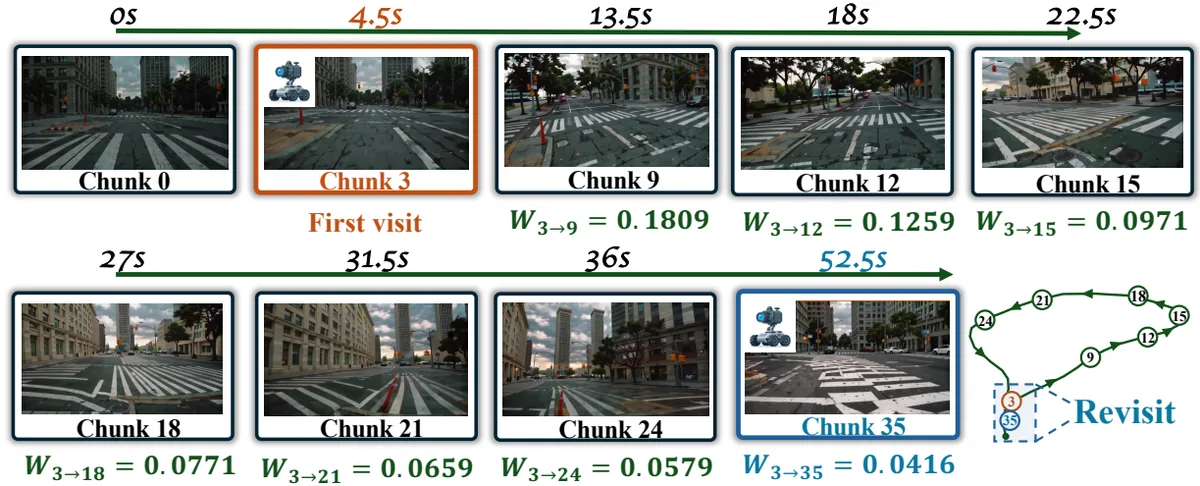
Key insight: GDN memory is updated according to “the passage of time,” but in a world model the relevance of information is determined not by time but by spatial/geometric proximity. This mismatch is the root cause of forgetting (source: §3).
New Approach: HLA-WM
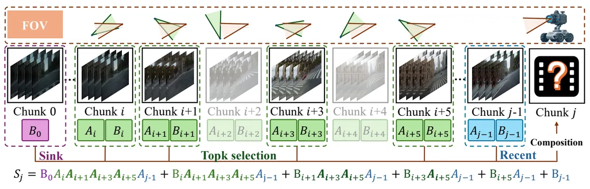
HLA-WM replaces the single accumulated GDN memory with a collection of independently addressable per-chunk memories (source: §4.1). It consists of three stages.
- Per-chunk GDN memory — Cache each time chunk as a single affine transition summary $(A_i, B_i)$.
- Geometry-based retrieval — Compute a frustum overlap score from the camera pose, intrinsics, and scene median depth to select relevant chunks.
- Selective state recomposition — Compose the selected summaries in temporal order to produce a query-specific recurrent state.
How It Works: A Concrete Walkthrough
1) GDN’s affine structure. The token-level GDN update is (source: §4.2, Eq. 4):
$$S_t = \gamma_t S_{t-1} + \beta_t (v_t - S_{t-1}k_t)\, k_t^{\top},$$where $k_t, v_t$ are the key and value projected from the current token, $\gamma_t$ is the memory decay, and $\beta_t$ is the delta update strength. Rearranging this gives the affine form $S_t = S_{t-1}A_t + B_t$, with
$$A_t = \gamma_t I - \beta_t k_t k_t^{\top},\qquad B_t = \beta_t v_t k_t^{\top}.$$Unrolling the $L$ tokens within a chunk $i$, the entire chunk can be represented by a single affine transition $(A_i, B_i)$. These summaries satisfy the associative law (source: Eq. 9):
$$(A_i, B_i) \star (A_j, B_j) = (A_i A_j,\; B_i A_j + B_j).$$This is the crux. Thanks to the associative law, any subset of history chunks can be recomposed efficiently without re-running the original visual tokens (source: §4.2).
2) Geometry retrieval. The overlap between each query chunk $q$ and history chunk $i$ is estimated from camera geometry alone, not from RGB or learned features. At a sampled pixel location $(u,v)$, the camera-space ray is formed as
$$r(u,v) = \Big[\tfrac{u-c_x}{f_x},\ \tfrac{v-c_y}{f_y},\ 1\Big]^{\top}$$and 3D points are scattered at three proxy depths around the scene median depth, $D = \{0.5d_{\text{med}}, d_{\text{med}}, 1.5d_{\text{med}}\}$, then projected into the camera view of the relative chunk to obtain the visible ratio $V$. The symmetric frustum overlap score is (source: §4.3, Eq. 12)
$$R(i,q) = \tfrac{1}{2}\big[V(i \to q) + V(q \to i)\big].$$3) Selection and recomposition. The first chunk is always retained as a sink, the recent chunks preserve local continuity, and the top $K$ of the remaining history by $R(i,q)$ are selected (source: Eq. 13)
$$I_q = I_{\text{sink}} \cup I_{\text{recent}} \cup \underset{i \in H_q}{\mathrm{TopK}}\; R(i,q),$$and the selected chunks are sorted in temporal order and composed to produce the query-specific history state (source: Eq. 17):
$$S_q^{\text{hist}} = S_0\, A_{\pi_q} + B_{\pi_q}.$$Concrete example. Return to the loop trajectory of Fig. 2. The camera goes Chunk 3 (first visit) → Chunk 4–34 (irrelevant distant departure) → Chunk 35 (revisit). When building $S_{35}$, the existing GDN passes the information written by Chunk 3 through the roughly 32 transitions of Chunk 4–34 in turn, eroding it down to $W_{3\to 35} = 0.0416$. HLA-WM, by contrast, detects when generating Chunk 35 that the frustum overlap with Chunk 3, $R(3, 35)$, is high, and selects Chunk 3’s summary $(A_3, B_3)$ along with the sink and recent context, composing them while skipping the transitions of Chunk 4–34. This vastly reduces the number of irrelevant transitions a distant but relevant memory is exposed to before reuse (source: §4.4).
Performance Validation: Main Results
Experiments were run on SANA-WM-Bench (80 trajectories each for simple/hard, 4 scene categories) and MBench-A (547 samples, 4 subsets), with the official 1.6B SANA-WM as the base model. HLA-WM modifies only the Stage-1 memory mechanism and does no fine-tuning (source: §5.1).
SANA-WM-Bench. In Stage-1 (the stage that directly modifies recurrent memory), HLA-WM improves both revisit consistency and camera control metrics across both splits (source: §5.2, Tab. 1):
| Pipeline | Metric | SANA-WM | HLA-WM | Δ | |—|—:|—:|—:| | Hard · Stage-1 | PSNR ↑ | 9.37 dB | 10.11 dB | +0.74 dB | | Hard · Stage-1 | SSIM ↑ | 0.1774 | 0.1997 | +0.0223 | | Hard · Stage-1 | LPIPS ↓ | 0.6044 | 0.5848 | −0.0196 | | Hard · Stage-1 | RotErr ↓ | 20.38° | 15.09° | −26.0% | | Simple · Stage-1 | PSNR ↑ | 9.18 dB | 9.91 dB | +0.73 dB | | Simple · Stage-1 | RotErr ↓ | 19.70° | 13.59° | −31.0% |
That is, the abstract’s headline numbers “PSNR +0.74 dB, rotation error −28.5%” combine the Stage-1 results for Hard (+0.74 dB, −26.0%) and Simple (−31.0%) (source: §Abstract, §5.2). Interestingly, the camera control metrics also improve. Preserved scene geometry reduces structural drift, providing a more stable spatial reference for camera-conditioned generation (source: §5.2).
Retained after downstream refinement. In bidirectional refinement all six metrics improve (PSNR +0.52/+0.46 dB, RotErr −22.0%/−20.1%), and revisit consistency improves consistently under causal AR refinement as well. However, in the refinement stage there is a trade-off in which some metrics worsen slightly depending on the mode (TransErr and CamMC for Simple) (source: §5.2, Tab. 1).
Generalization: MBench-A. Across all 547 samples, PSNR, SSIM, and LPIPS improve consistently in all three inference modes. In Stage-1 the largest gains appear: PSNR +0.84 dB, SSIM +0.0303, LPIPS −0.0428 (source: §5.2, Tab. 2). The gains are not concentrated in a specific subset; all three metrics improve simultaneously across all 12 mode–subset combinations (source: Appx. A.8.2).
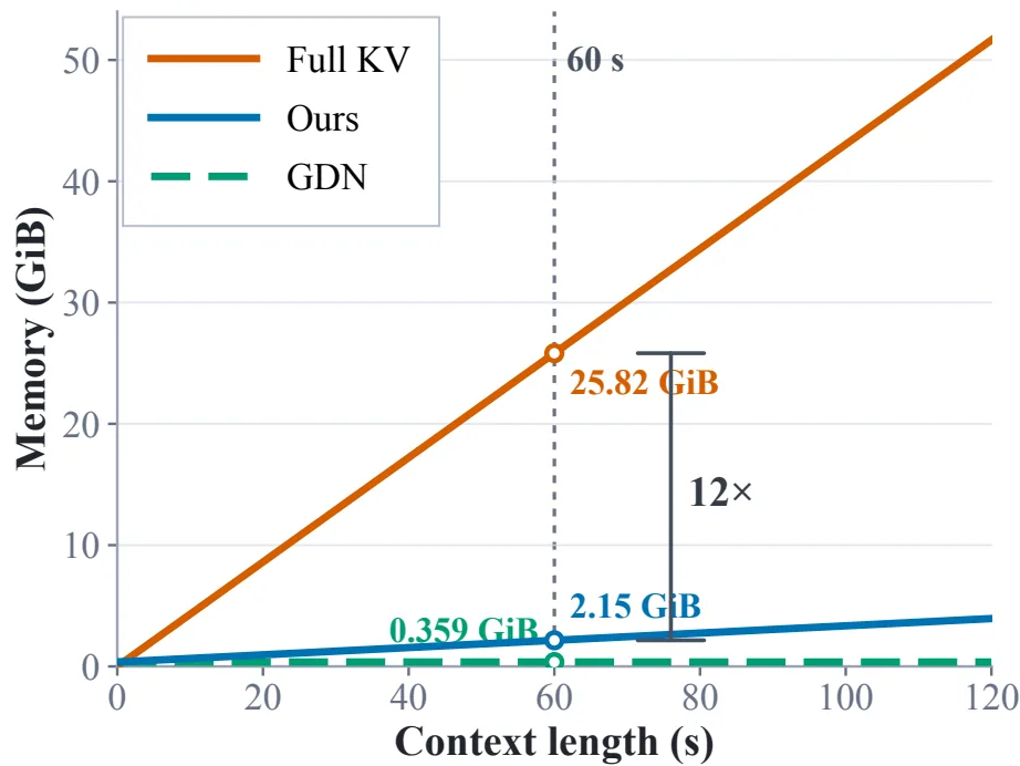
Efficiency. HLA-WM offers a practical compromise between Full KV attention and recurrent linear attention. Because the history is cached in chunks rather than tokens, memory scales with the number of chunks rather than the number of tokens. On a 60-second context it uses only 2.15 GiB (a 12× reduction over Full KV) while incurring a throughput loss of at most 1.6% (source: §5.2, Fig. 4).
Key ablations. The authors answer two questions (source: Appx. A.3–A.5).
- Which components matter? Removing the sink, disabling transition selection (“w/o Select A”), disabling write selection (“w/o Select B”), and removing turn-aware recent context all degrade revisit consistency and camera control. In particular, leaving in irrelevant intermediate transitions drops PSNR and SSIM substantially, supporting the claim that “irrelevant transitions are the cause of forgetting” (source: Appx. A.3, Tab. 3).
- Which matters more, GDN recomposition or KV alignment? GDN-only yields a far larger gain than KV-only, and combining the two gives the best performance. In the Hard trajectories of bidirectional refinement, GDN-only raises SSIM but worsens RotErr from 13.17° to 33.04°, showing a “memory-path mismatch”; applying the same selection to the KV cache stabilizes it again (source: Appx. A.4, Tab. 4).
Retrieval budget and selection strategy. Surprisingly, $K{=}1$ (the single most relevant history chunk) is best on PSNR, SSIM, and LPIPS. Retrieving more gives no consistent improvement (source: Appx. A.5, Tab. 6). Also, geometry-based selection gives better revisit consistency than heuristics such as Random, Recent, and Uniform, showing that beyond “broad temporal coverage,” explicitly choosing view-relevant history provides additional benefit (source: Appx. A.6, Tab. 7).
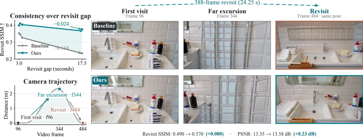
Effect of revisit interval. The gain grows with the revisit interval (PSNR improvement rises from +0.375 dB at short intervals <10s to +0.992 dB at long intervals ≥40s). This result aligns exactly with the method’s intent: the benefit of selective long-term memory is most pronounced for the “heavily forgotten” long-range revisits (source: Appx. A.7, Fig. 6).
Our Perspective: Strengths, Limitations, and Why This Work Matters
Strengths. The most striking aspect is the practicality of being training-free. It leaves the pretrained 1.6B model untouched and only changes how memory is accessed at inference time to raise long-range consistency. Exploiting GDN’s affine structure analytically to scale memory as $O(\text{chunks})$ rather than $O(\text{tokens})$ while simultaneously achieving a 12× reduction and a throughput loss of around 1.6% is a strong demonstration of the viability of the idea of “selectively addressable recurrent memory” (source: §4.4, Fig. 4). The GDN-only vs KV-only ablation, which isolates that “recurrent state recomposition is the main driver,” is also analytically clean (source: Appx. A.4).
Limitations. As the authors explicitly acknowledge, the training-free property itself constrains the ceiling. Retrieval relies only on camera geometry and FOV overlap and does not model occlusion, visibility, or semantic relevance (source: §6). We would point to three additional limitations. First, retrieval assumes a prescribed camera trajectory, whereas in open-loop generation by a real agent the pose must be estimated separately, and that error propagates into retrieval quality. Second, the “fixed 24-frame chunk” and “sink 1 + recent 1 + Top-1” design are values tuned on the specific SANA-WM-Bench and MBench-A pipelines, so robustness to different chunking and fps remains open. Third, the result that $K{=}1$ is optimal also means, conversely, that “richer retrieval does not help,” suggesting a representational limit in the retrieval signal itself (source: Appx. A.5).
Why this work matters. This paper connects the LLM KV-cache compression and long-context literature with the video world model literature. On the spectrum between a “full history cache” and a “single compressed state,” it offers a third point — selective recomposition using geometric information as an addressing signal — and shows that it works without training. As video world models grow longer, “how to address memory” will become the bottleneck, and this paper provides one concrete, measurable answer to that question.
What’s Next?: The Road Ahead
The authors propose integrating selective state retrieval into training and richer or learned retrieval signals that include occlusion, visibility, and semantic relevance as future directions (source: §6). Beyond these, the directions we would look forward to are as follows.
- Combining with a learned router. For now, camera geometry is a “free” addressing signal, but it has limits for semantic revisits (the reappearance of the same object rather than the same place). A hybrid in which geometric signals serve as a prior and a lightweight router corrects them is natural.
- Occlusion-aware retrieval. Frustum overlap cannot see “behind walls.” Adding depth-buffer or occupancy signals could reduce occlusion errors in indoor scenes.
- Automating chunking and the retrieval budget. Instead of a fixed 24 frames and Top-1, dynamically adjusting the chunk size and $K$ based on scene change rate or motion magnitude could achieve a better efficiency–quality trade-off.
- Deeper optimization of the recomposition kernel. The forward scan the authors implemented on top of a Triton kernel is a starting point. Batching and memory-layout optimizations could reduce that 1.6% throughput loss further (source: §4.4, Appx. A.2).
In summary, HLA-WM starts from a clear diagnosis of “the forgetting of recurrent linear attention,” offers an elegant and practical solution — geometry-based selective recomposition — and robustly validates its effectiveness on two benchmarks. By driving this much long-range consistency improvement without any training, this work will be an important stepping stone toward efficient long-horizon world models.
Tables from the paper
Tables converted mechanically from the arXiv e-print LaTeX source. The numbers are the paper’s own and did not pass through a model.
Expand all original paper tables
Table 1. Main results on SANA-WM-Bench under different generation stages and refinement modes. We report revisit consistency, camera controllability, and inference throughput. Best results within each setting are shown in bold.
| Pipeline | Method | Revisit Consistency PSNR $\uparrow$ | Revisit Consistency SSIM $\uparrow$ | Revisit Consistency LPIPS $\downarrow$ | Camera Control RotErr ($^\circ$) $\downarrow$ | Camera Control TransErr $\downarrow$ | Camera Control CamMC $\downarrow$ | Efficiency FPS $\uparrow$ |
|---|---|---|---|---|---|---|---|---|
| Simple-Trajectory Split | ||||||||
| Stage-1 | SANA-WM | 9.18 | 0.1729 | 0.6327 | 19.7040 | 2.2625 | 2.3974 | 22.403 |
| HLA-WM | 9.91 | 0.1999 | 0.6049 | 13.5864 | 2.0928 | 2.1798 | 22.053 | |
| Stage-1 + AR Refine | SANA-WM | 14.44 | 0.2770 | 0.5738 | 20.9315 | 2.1587 | 2.3121 | 8.280 |
| HLA-WM | 14.82 | 0.2872 | 0.5682 | 20.2933 | 2.1910 | 2.3240 | 8.211 | |
| Stage-1 + Bi. Refine | SANA-WM | 13.04 | 0.2945 | 0.5786 | 11.3848 | 1.9893 | 2.0545 | 7.701 |
| HLA-WM | 13.56 | 0.3148 | 0.5614 | 8.8823 | 1.8637 | 1.9127 | 7.700 | |
| Hard-Trajectory Split | ||||||||
| Stage-1 | SANA-WM | 9.37 | 0.1774 | 0.6044 | 20.3759 | 1.9952 | 2.1507 | 22.403 |
| HLA-WM | 10.11 | 0.1997 | 0.5848 | 15.0887 | 1.8388 | 1.9482 | 22.053 | |
| Stage-1 + AR Refine | SANA-WM | 14.12 | 0.2719 | 0.5621 | 25.6330 | 2.0099 | 2.2079 | 8.280 |
| HLA-WM | 14.47 | 0.2812 | 0.5557 | 22.0165 | 1.9351 | 2.1043 | 8.211 | |
| Stage-1 + Bi. Refine | SANA-WM | 13.05 | 0.2972 | 0.5468 | 13.1713 | 1.6649 | 1.7694 | 7.701 |
| HLA-WM | 13.51 | 0.3142 | 0.5384 | 10.5268 | 1.5449 | 1.6230 | 7.700 |
Table 2. Component ablation on the Hard-Trajectory split using Stage 1 outputs. Best results are shown in bold.
| Variant | Revisit Consistency PSNR $\uparrow$ | Revisit Consistency SSIM $\uparrow$ | Revisit Consistency LPIPS $\downarrow$ | Camera Control RotErr ($^\circ$) $\downarrow$ | Camera Control TransErr $\downarrow$ | Camera Control CamMC $\downarrow$ |
|---|---|---|---|---|---|---|
| HLA-WM | 10.11 | 0.1997 | 0.5848 | 15.0887 | 1.8388 | 1.9482 |
| w/o Sink | 9.71 | 0.1867 | 0.6019 | 15.9351 | 1.9326 | 2.0531 |
| w/o Select $A$ | 9.61 | 0.1887 | 0.5901 | 15.2426 | 1.8552 | 2.0562 |
| w/o Select $B$ | 9.64 | 0.1892 | 0.5921 | 15.2326 | 1.9830 | 2.0564 |
| w/o Turn-aware | 9.96 | 0.1917 | 0.5876 | 15.1784 | 2.1096 | 1.9899 |
Table 3. Ablation of GDN-state recomposition and KV-cache alignment on SANA-WM-Bench under Top-$1$ retrieval. Best results within each split and inference setting are shown in bold.
| Pipeline | Method | PSNR $\uparrow$ | SSIM $\uparrow$ | LPIPS $\downarrow$ | RotErr ($^\circ$) $\downarrow$ | TransErr $\downarrow$ | CamMC $\downarrow$ |
|---|---|---|---|---|---|---|---|
| Simple-Trajectory Split | |||||||
| Stage 1 | Baseline | 9.18 | 0.1729 | 0.6327 | 19.7040 | 2.2625 | 2.3974 |
| GDN-only | 9.45 | 0.1812 | 0.6219 | 17.9934 | 2.2832 | 2.4083 | |
| KV-only | 9.50 | 0.1866 | 0.6149 | 14.4283 | 1.9569 | 2.0556 | |
| HLA-WM | 9.91 | 0.1999 | 0.6049 | 13.5864 | 2.0928 | 2.1798 | |
| Stage 1 + AR Refine | Baseline | 14.44 | 0.2770 | 0.5738 | 20.9315 | 2.1587 | 2.3121 |
| GDN-only | 14.65 | 0.2784 | 0.5687 | 21.2344 | 2.3596 | 2.5147 | |
| KV-only | 13.88 | 0.2703 | 0.5812 | 20.9084 | 2.2087 | 2.3662 | |
| HLA-WM | 14.82 | 0.2872 | 0.5682 | 20.2933 | 2.1910 | 2.3240 | |
| Stage 1 + Bi. Refine | Baseline | 13.04 | 0.2945 | 0.5786 | 11.3848 | 1.9893 | 2.0545 |
| GDN-only | 13.26 | 0.2998 | 0.5746 | 10.7564 | 1.8627 | 1.9310 | |
| KV-only | 13.17 | 0.2999 | 0.5762 | 9.6939 | 1.8866 | 1.9417 | |
| HLA-WM | 13.56 | 0.3148 | 0.5614 | 8.8823 | 1.8637 | 1.9127 | |
| Hard-Trajectory Split | |||||||
| Stage 1 | Baseline | 9.37 | 0.1774 | 0.6044 | 20.3759 | 1.9952 | 2.1507 |
| GDN-only | 9.78 | 0.1890 | 0.5929 | 20.0838 | 1.9502 | 2.1075 | |
| KV-only | 9.52 | 0.1805 | 0.6000 | 13.3992 | 1.7635 | 1.8616 | |
| HLA-WM | 10.11 | 0.1997 | 0.5848 | 15.0887 | 1.8388 | 1.9482 | |
| Stage 1 + AR Refine | Baseline | 14.12 | 0.2719 | 0.5621 | 25.6330 | 2.0099 | 2.2079 |
| GDN-only | 14.35 | 0.2797 | 0.5576 | 23.1860 | 1.9519 | 2.1296 | |
| KV-only | 13.54 | 0.2599 | 0.5721 | 24.1145 | 2.0425 | 2.2302 | |
| HLA-WM | 14.47 | 0.2812 | 0.5557 | 22.0165 | 1.9351 | 2.1043 | |
| Stage 1 + Bi. Refine | Baseline | 13.05 | 0.2972 | 0.5468 | 13.1713 | 1.6649 | 1.7694 |
| GDN-only | 13.49 | 0.3304 | 0.5601 | 33.0406 | 2.1843 | 2.4584 | |
| KV-only | 13.26 | 0.3047 | 0.5469 | 11.4688 | 1.5860 | 1.6696 | |
| HLA-WM | 13.51 | 0.3142 | 0.5384 | 10.5268 | 1.5449 | 1.6230 |
Table 4. Ablation of GDN-state recomposition and KV-cache alignment on MBench-A under Top-$1$ retrieval. Best results within each inference setting are shown in bold.
| Pipeline | Method | PSNR $\uparrow$ | SSIM $\uparrow$ | LPIPS $\downarrow$ |
|---|---|---|---|---|
| Stage 1 | Baseline | 10.17 | 0.2545 | 0.6251 |
| GDN-only | 10.61 | 0.2626 | 0.6052 | |
| KV-only | 10.43 | 0.2606 | 0.6091 | |
| HLA-WM | 11.01 | 0.2848 | 0.5823 | |
| Causal AR Refine | Baseline | 12.36 | 0.2996 | 0.6554 |
| GDN-only | 12.57 | 0.3064 | 0.6492 | |
| KV-only | 12.35 | 0.3016 | 0.6547 | |
| HLA-WM | 12.73 | 0.3122 | 0.6447 | |
| Bidirectional Refine | Baseline | 12.94 | 0.3310 | 0.5597 |
| GDN-only | 13.28 | 0.3389 | 0.5477 | |
| KV-only | 13.04 | 0.3325 | 0.5563 | |
| HLA-WM | 13.52 | 0.3431 | 0.5470 |
Table 5. Ablation on the retrieval budget $K$ on the Hard-Trajectory split using Stage 1 outputs. Best results are shown in bold.
| $K$ | Revisit Consistency PSNR $\uparrow$ | Revisit Consistency SSIM $\uparrow$ | Revisit Consistency LPIPS $\downarrow$ | Camera Control RotErr ($^\circ$) $\downarrow$ | Camera Control TransErr $\downarrow$ | Camera Control CamMC $\downarrow$ |
|---|---|---|---|---|---|---|
| $1$ | 10.11 | 0.1997 | 0.5848 | 15.0887 | 1.8388 | 1.9482 |
| $3$ | 10.06 | 0.1973 | 0.5865 | 14.1537 | 1.7658 | 1.8661 |
| $4$ | 10.00 | 0.1936 | 0.5885 | 12.2795 | 1.6985 | 1.7832 |
| $5$ | 9.89 | 0.1886 | 0.5915 | 11.5435 | 1.7200 | 1.7970 |
Table 6. Comparison of historical state selection strategies on Hard80 under Stage 1 inference with $K=4$. Higher PSNR and SSIM are better, while lower LPIPS and camera errors are better.
| Selection Policy | PSNR $\uparrow$ | SSIM $\uparrow$ | LPIPS $\downarrow$ | RotErr ($^\circ$) $\downarrow$ | TransErr $\downarrow$ | CamMC $\downarrow$ |
|---|---|---|---|---|---|---|
| Random | 9.70 | 0.1864 | 0.6049 | 14.1883 | 1.7822 | 1.8924 |
| Recent | 9.29 | 0.1696 | 0.6179 | 27.6876 | 2.0142 | 2.2408 |
| Uniform | 9.91 | 0.1910 | 0.5957 | 12.3324 | 1.6881 | 1.7838 |
| HLA-WM | 10.00 | 0.1936 | 0.5885 | 12.2795 | 1.6985 | 1.7832 |
Table 7. Category-level results on SANA-WM-Bench using Stage 1 outputs. Best results within each category are shown in bold.
| Category | Method | PSNR $\uparrow$ | SSIM $\uparrow$ | LPIPS $\downarrow$ | RotErr ($^\circ$) $\downarrow$ | TransErr $\downarrow$ | CamMC $\downarrow$ |
|---|---|---|---|---|---|---|---|
| Simple-Trajectory Split | |||||||
| Game Style | SANA-WM | 9.85 | 0.2070 | 0.6197 | 16.5064 | 1.9242 | 2.0482 |
| HLA-WM | 11.06 | 0.2639 | 0.5866 | 12.8640 | 2.0047 | 2.0939 | |
| Indoor | SANA-WM | 9.38 | 0.2105 | 0.6576 | 38.6940 | 1.6993 | 2.0227 |
| HLA-WM | 10.05 | 0.2338 | 0.6306 | 29.0323 | 1.6196 | 1.8481 | |
| Outdoor City | SANA-WM | 8.96 | 0.1323 | 0.6390 | 12.2424 | 2.0782 | 2.1372 |
| HLA-WM | 9.25 | 0.1561 | 0.6240 | 5.9851 | 1.5976 | 1.6170 | |
| Outdoor Nature | SANA-WM | 8.52 | 0.1419 | 0.6145 | 11.3733 | 3.3483 | 3.3814 |
| HLA-WM | 9.29 | 0.1459 | 0.5785 | 6.4643 | 3.1493 | 3.1603 | |
| Hard-Trajectory Split | |||||||
| Game Style | SANA-WM | 9.84 | 0.2023 | 0.5823 | 14.2161 | 1.8745 | 1.9719 |
| HLA-WM | 11.41 | 0.2550 | 0.5505 | 14.3713 | 1.8250 | 1.9349 | |
| Indoor | SANA-WM | 9.22 | 0.2085 | 0.6390 | 36.5361 | 1.2446 | 1.6297 |
| HLA-WM | 9.63 | 0.2305 | 0.6330 | 26.6061 | 1.0675 | 1.3277 | |
| Outdoor City | SANA-WM | 9.17 | 0.1463 | 0.6206 | 16.0176 | 1.8409 | 1.9254 |
| HLA-WM | 9.56 | 0.1611 | 0.6122 | 9.9119 | 1.6669 | 1.7070 | |
| Outdoor Nature | SANA-WM | 9.23 | 0.1526 | 0.5756 | 14.7337 | 3.0208 | 3.0760 |
| HLA-WM | 9.84 | 0.1521 | 0.5437 | 9.4654 | 2.7958 | 2.8233 |
Table 8. Category-level results on SANA-WM-Bench after causal AR refinement. Best results within each category are shown in bold.
| Category | Method | PSNR $\uparrow$ | SSIM $\uparrow$ | LPIPS $\downarrow$ | RotErr ($^\circ$) $\downarrow$ | TransErr $\downarrow$ | CamMC $\downarrow$ |
|---|---|---|---|---|---|---|---|
| Simple-Trajectory Split | |||||||
| Game Style | SANA-WM | 15.19 | 0.3225 | 0.5582 | 19.8894 | 2.1729 | 2.3106 |
| HLA-WM | 15.79 | 0.3505 | 0.5492 | 16.5280 | 2.0506 | 2.1496 | |
| Indoor | SANA-WM | 13.64 | 0.3127 | 0.6013 | 35.3855 | 1.5308 | 1.8652 |
| HLA-WM | 14.08 | 0.3172 | 0.5956 | 34.3931 | 1.6263 | 1.9040 | |
| Outdoor City | SANA-WM | 14.21 | 0.2353 | 0.5803 | 15.1111 | 1.9558 | 2.0376 |
| HLA-WM | 14.26 | 0.2510 | 0.5777 | 14.4444 | 1.9104 | 1.9801 | |
| Outdoor Nature | SANA-WM | 14.70 | 0.2375 | 0.5555 | 13.3400 | 2.9753 | 3.0350 |
| HLA-WM | 15.13 | 0.2302 | 0.5503 | 15.8077 | 3.1768 | 3.2625 | |
| Hard-Trajectory Split | |||||||
| Game Style | SANA-WM | 14.95 | 0.3220 | 0.5269 | 23.5136 | 1.8901 | 2.0707 |
| HLA-WM | 15.73 | 0.3398 | 0.5140 | 18.0932 | 1.8923 | 2.0223 | |
| Indoor | SANA-WM | 13.81 | 0.3003 | 0.5923 | 35.8487 | 1.2361 | 1.6201 |
| HLA-WM | 13.71 | 0.3139 | 0.5920 | 30.6444 | 1.1457 | 1.4865 | |
| Outdoor City | SANA-WM | 13.56 | 0.2507 | 0.5812 | 20.0231 | 1.8331 | 1.9407 |
| HLA-WM | 13.74 | 0.2570 | 0.5877 | 19.7262 | 1.8103 | 1.9228 | |
| Outdoor Nature | SANA-WM | 14.18 | 0.2147 | 0.5478 | 23.1465 | 3.0804 | 3.2001 |
| HLA-WM | 14.71 | 0.2143 | 0.5290 | 19.6023 | 2.8921 | 2.9858 |
Figures in this post are taken from the original arXiv:2610.05739 (CC BY 4.0). Only size and format were changed.
Comments