Phase Sensitivity: The ‘Periodic Weakness’ Created by Chunked KV-Cache Compression
TL;DR — In models that use chunked KV-cache compression (such as the DeepSeek-V4 family), the same information can vary in retrieval performance by up to 40pp periodically depending on its ‘phase’ relative to the compression window boundary. Average benchmark scores completely hide this weakness.
Core Idea
The bottleneck of long-context reasoning is the KV cache. Memory and attention costs grow in proportion to context length (source: §1). To address this, models like DeepSeek-V4 use chunked KV-cache compression. Consecutive tokens are grouped into fixed-size windows, each window is summarized into a smaller number of cache entries, and long-range retrieval is performed using those summaries (source: §1).
The insight of this paper starts here. Compression forces a periodic structure in which a new window begins every $S$ tokens onto the context. $S$ is the compression stride. Each token then acquires a new coordinate besides absolute position: its phase (source: §1):
$$\text{phase} = t \bmod S$$Merely shifting the input by a few tokens leaves the content and relative positions unchanged, yet which tokens get grouped into the same window changes. That is, the same information is compressed differently depending on phase, and can therefore be preserved with different fidelity.
The authors define it this way. For stride $S$, the phase of the key-value pair starting at position $t$ is $t \bmod S$. When some retrieval metric (accuracy, probability of the correct answer, etc.) varies systematically with the phase of the information, retrieval is said to exhibit phase sensitivity (source: §2).
The core claim is summarized in this one sentence. “In models that use chunked KV-cache compression, there exists a periodic retrieval failure (periodic weakness) invisible in average scores, and its period matches the compression stride.”
Background: The Problem They Solved
The cost of the KV cache grows in proportion to context length. Roughly, for a model with $L$ layers, $H$ heads, and head dimension $d_\text{head}$, at sequence length $\text{seq}$ and batch size $\text{batch}$, the cache size grows as follows:
$$ \text{KV-Cache(GB)} \approx \frac{2 \cdot L \cdot H \cdot d_\text{head} \cdot \text{seq} \cdot \text{batch} \cdot \text{bytes/elt}}{10^9} $$The family of learned compression memory approaches emerged to reduce this cost. Compressive Transformer, LoMA, Activation Beacon, CAT, along with sparse attention (NSA, MOBA, DeepSeek-V4’s CSA) and cache eviction (H2O, SnapKV), all share the same goal (source: §6).
Yet existing evaluation methods have a blind spot. “Lost in the Middle” showed that depth in the context determines retrieval quality, and RULER showed that easy needle tests overestimate the practically usable context length (source: §6). What this paper focuses on is an entirely different dimension. Not the context depth or query position of information, but its phase relative to compression window boundaries — a microscopic coordinate that repeats every stride.
What the authors found is surprising. The retrieval performance of the same information fluctuates periodically with this phase. And this is completely masked by average metrics.
New Approach: Phase Sensitivity + Phase Specialization
This paper does not propose a new model or a new architecture. Instead, it is an analysis paper that defines a new failure mode and identifies its origin mechanistically and theoretically. The contributions fall broadly into three categories (source: §1, §3, §4, §5).
Identification of a new failure mode (empirical discovery). It is the first to report ‘phase sensitivity,’ in which retrieval accuracy varies periodically with phase in chunked KV compression models. It reproduces in DeepSeek-V4, V4.1, and in all compression models the authors pretrained themselves.
Mechanism identification (causal intervention). Through causal interventions such as KV head knockout and gate cycling, it demonstrates phase specialization, in which different heads contribute asymmetrically to retrieval at different phases.
Theoretical explanation (optimization dynamics). On an idealized bigram retrieval task, it shows that concentration of the compression gate is the optimum, and proves as a theorem that gradient flow freezes that concentration statically.
What sets this apart from prior work is that it abandons the lens of ‘average accuracy.’ It digs into the fact that, even when benchmark scores are the same, a periodically repeating positional failure hides within.
How It Works: A Concrete Example
How Chunk Compression Is Done
The compression kernel used in the controlled experiments makes the behavior clear (source: §3). Let the hidden state at offset $i$ ($0 \le i < W$) in window $j$ of window size $W$ be $h_{j,i} \in \mathbb{R}^d$. Each offset determines “what to contribute” via a payload map $C_i$, and “how strongly to enter” via compression gates $Z_i$, $b_i$. In the key branch, the gate logit is:
$$ s_{j,i}^{K} = Z_{i}^{K} h_{j,i} + b_{i}^{K} $$A softmax is taken over the whole window to produce gate scores, which are multiplied against the payload and summed:
$$ \alpha_{j,i}^{K} = \frac{\exp(s_{j,i}^{K})}{\sum_{u=0}^{W-1} \exp(s_{j,u}^{K})}, \qquad \widehat{K}_j = \sum_{i=0}^{W-1} \alpha_{j,i}^{K} \odot \left( C_i^K h_{j,i} \right) $$The key point is that this compression happens before knowing the query. Without knowing which information will need to be recalled later, every window must be summarized in a ‘query-agnostic’ way. This structure gives rise to periodicity.
Toy Example: 8-Token Window, Stride 8
Imagine a model with $S=8$. A new window starts at positions $0,8,16,\dots$. A token at position $t$ has phase $t \bmod 8$. That is, $t=0$ and $t=8$ both have phase $0$, and $t=1$ and $t=9$ both have phase $1$.
Now suppose the key-value pair “key: banana, value: yellow” is at position $t$. At retrieval, we throw in the query banana and must recover yellow.
- If $t=7$, the key falls at the last offset of window $j$, and the value
yellowfalls at the first offset of the next window $j{+}1$. Since the key and value are split across the window boundary, both cannot fit inside a single compression entry. Intuitively, retrieval is difficult (source: §3). - From $t=0$ to $t=6$, the key and value are inside the same window. And yet in experiments, accuracy differs by more than 50pp across these phases (source: §3). In other words, the boundary alone cannot explain the entire period.
This dual asymmetry — “the case crossing the boundary vs. the difference that persists even inside the window” — is the analytical axis of this paper.
Gates Learn the Phase
The clue to phase specialization lies in the gates. Because gate scores depend on the input, they can concentrate in two ways (source: §4).
- Static concentration: whatever input arrives, the same offset is always preferred. → Fixed to a particular phase.
- Input-dependent concentration: the preferred offset changes with content. → Independent of phase.
These two are distinguished by the effective number of offsets. Defined as $\exp(H(\alpha))$ for entropy $H$, it is $1$ for a one-hot and $W$ for a uniform distribution. Right after initialization, all gates are close to uniform ($\exp(H(\mathbb{E}[\alpha])) \approx 8$), but as pretraining proceeds, some heads slide down the diagonal and form static concentration (source: §4).
Specifically, in the reference model (W8/S8), the gates of layers 9, 10, and 14 form peaks at the late, middle, and early offsets of the window, respectively, and the value gates form peaks one offset after that. It looks as though a single head takes sole charge of a key-value pair (bigram) (source: §4). This peak phase exactly matches the phase where that head’s knockout loss is concentrated.
Performance Validation: Key Results
The Periodic Weakness of the DeepSeek-V4 Family
The most striking evidence is code completion. When DeepSeek-V4-Flash-Base is asked to complete the type cast of its own inference code (an FP8 quantization function), a decorative docstring was prepended and only its length $L$ was varied from 24 to 39 tokens. The code is identical, yet the top-1 prediction flips periodically. The probability difference $P(8) - P(32)$ between the correct answer 8 and the wrong answer 32 oscillates from $-0.79$ to $+0.95$, and the flip repeats every 4 tokens (source: §2, Fig. headline). This period of 4 is exactly the stride $S=4$ of DeepSeek-V4 CSA. The same phenomenon appears with period 2 in DeepSeek-V4.1-Flash, whose stride is $S=2$, and in DeepSeek-V3.1-Base, which has no chunk compression, 32 comes out on top in only 4 of 64 inputs, so it effectively disappears (source: §2).
What systematizes this is a NIAH (needle-in-a-haystack) retrieval experiment at 128K context. 16k key-value pairs are inserted into a 128K-token prompt, and the original key value somewhere in the middle must be recovered (source: §2). Looking at accuracy by the remainder of the original key’s position divided by 8 (phase group), it reaches up to 40.2pp in the base checkpoint (source: §2, Fig. v4_niah). Although post-training raises accuracy and narrows the gap, the gap remains 19.14pp for DeepSeek-V4-Flash-0731 and 14.84pp for DeepSeek-V4-Pro-0813 (source: Tab. v4-niah-residue-accuracy). Even V4.1-Flash, with the smallest gap, is at 6.09pp, and all four even phase groups sit above all four odd groups (source: §2).
Controlled Pretraining: Confirming Compression Is the Cause
DeepSeek-V4 differs from a standard transformer in many ways besides chunk compression, so one cannot retrain it without compression to check whether the periodicity disappears. So the authors pretrained from scratch a family of models using Qwen3-0.6B as the backbone, with KV compression as the sole architectural change. A total of 26 runs (23 compressed + 3 full-attention baselines) were trained to step 47,518 (source: §3, Tab. controlled-sweep-results).
The result is clear. Every compression model fluctuates periodically in line with the stride, and the full-attention baseline is flat (source: §3).
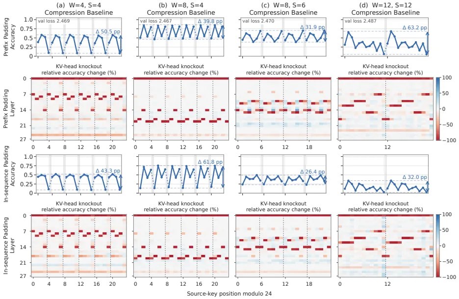
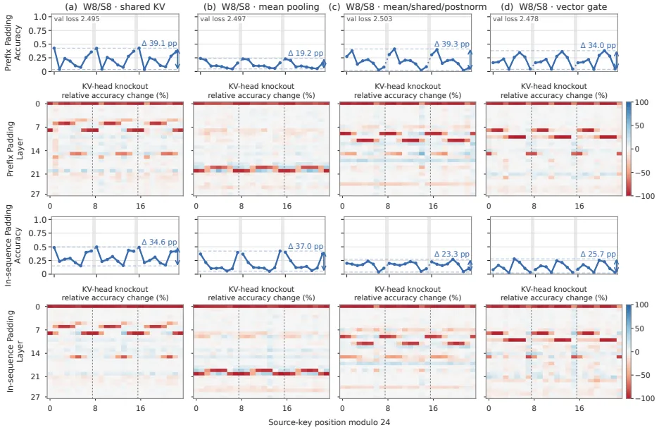
In particular, the period itself follows the stride. With window $W=8$ and strides $S\in\{4,6,8\}$, the periods are about 4, 6, and 8 tokens respectively, and about 12 tokens for $W{=}12/S{=}12$ (source: §3). And this phenomenon remains even without RoPE or learned gates. Replacing the gates with uniform mean pooling, or removing positional encoding, phase sensitivity persists (source: §3).
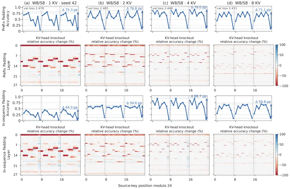
The most chilling number is ‘how much the average metric hides this difference.’ A W8/S8 compression model with 8 KV heads nearly approaches the full-attention baseline (61.1%) in average accuracy (59.4%) and validation loss, yet its worst phase-group accuracy is only 9.9%. The baseline’s lowest is 58.4% (source: §3, Tab. controlled-sweep-results). The Prefix Padding gap reaches up to 78pp in compression models, whereas the baseline is at most 6.1pp (source: §3).
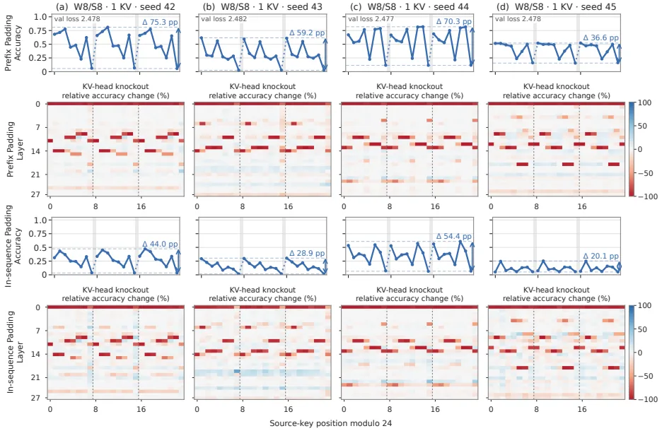
This phenomenon is robust to seeds. Changing the seed changes the pattern of per-phase accuracy, but the periodic weakness itself reproduces across all seeds (source: Appx).
Mechanism: Phase Specialization
To find the cause, KV head knockout was performed. The output of one head at a time is replaced with its mean across multiple prompts (mean replacement), erasing “the information specific to this prompt” (source: §4). In the full-attention baseline, the loss of each layer appears as horizontal stripes spread evenly across all phases. In compression models, by contrast, the loss is concentrated on particular phases, and each head shows a different phase-dependent pattern (source: §4, Fig. phase-knockouts). The same pattern repeats with a 4-token period in DeepSeek-V4-Flash-Base as well.
Causality is then confirmed with a gate cycling intervention. Cycling the per-offset parameters of a statically concentrated gate by $k$ offsets shifts the accuracy pattern by roughly $k$ phases as well (source: §4). This shows that the learned gate preference is the cause of the per-phase retrieval asymmetry.
Theory: Why Gates Concentrate on Phase
Finally, the authors ask “why” with an idealized induction task. In a context where $LS$ tokens are divided into chunks of stride $S$, when a query repeats a token, the task is to predict its successor token (source: §5). Each head summarizes a chunk into a single compressed key/value. Two theorems follow (source: §5).
Theorem 1 (The optimal compression is concentrated). For a sufficiently large vocabulary $N$ and small error $\varepsilon$, the global minimizer concentrates the key weight on a single position $r$ and the value weight on $r{+}1$ as one-hots across all contexts, chunks, and heads. That is, even without knowing the query in advance, the loss prefers the most concentrated compression.
Theorem 2 (Gradient flow creates static concentration). Gradient flow starting from a small random initialization converges each head $h$ to a fixed position $r_h$, so that the key gate becomes a one-hot at $r_h$ and the value gate a one-hot at $r_h{+}1$. In Theorem 1 the chosen position could differ per input, but in Theorem 2 training fixes it per head.
This matches exactly the adjacent preference observed earlier in layers 9, 10, and 14 — “the key at a particular offset, the value at the next offset” (source: §5).
Our Perspective: Strengths, Limitations, and Why This Matters
Strengths. The greatest value of this paper is that it cracks the inertia of ‘average accuracy.’ The fact that a periodic failure of up to 40pp can hide inside a model whose benchmark scores are the same has direct implications for the evaluation protocols of every long-context model that uses chunk compression. Methodologically it is clean too. It goes beyond manual observation of a single model and stacks four layers: (1) a large family of commercial models, (2) pretraining with a single controlled variable, (3) causal intervention, and (4) theoretical theorems. In particular, the experimental design of “shifting the input by a few tokens to change the phase of the same information” is easy to reproduce and could become a standard tool in this field.
Limitations. As the authors themselves state, the mechanistic conclusions are strongest in the controlled small-scale setting. They have not established a universal cause in large heterogeneous models (source: §7). A more important unresolved point is the duality. Since gate cycling cannot restore the boundary phase (the case where the key and value cross the window), it has not unified the boundary asymmetry and the within-window asymmetry into a single explanation (source: §7). The theory too is confined to the idealization of a bigram induction task and does not extend to the complex loss landscape of real pretraining. Many quantitative metrics are also concentrated on controlled tasks like NIAH and code completion, so the felt impact in real downstream applications remains open.
Why this matters. In long-context reasoning, where performance optimization is progressing rapidly, this paper pinpoints with concrete coordinates that “wherever you cut cost, a price hides somewhere.” Even a compression design that succeeds in raising the average can lose reliability depending on which phase the information lands in. This raises new questions for both evaluation methodology (phase-decomposed measurement rather than averages) and architecture design (phase homogenization).
What’s Next?: The Road Ahead
The most practical task the authors leave behind is phase homogenization. Whether explicit coordination across heads and layers can even out per-phase retrieval quality, without sacrificing average performance or compression efficiency, remains open (source: §7).
In our view, the natural next steps are threefold.
Standardization of evaluation protocols. Add a procedure to existing long-context benchmarks (Lost in the Middle, RULER, etc.) that ‘shifts the input by $k$ tokens and measures per phase,’ and establish the practice of reporting the minimum and the gap alongside the average.
Exploring robustness implications. As the authors state, it is still unverified whether a meaning-preserving input shift changes response refusal or compliance, and whether that change tracks the compression phase (source: §7). The connection to safety-related behaviors such as prompt injection, jailbreaking, and consistency is an urgent question.
Design-level responses. If the static concentration of gates is one cause, it is worth experimenting with a loss term that regularizes it or derives a phase-independent compression operator, or with input preprocessing that mixes phases to spread out (pipeline) the weakness. The theoretical theorem says that “training naturally prefers concentration,” so simply training longer will not solve it.
Ultimately, the lesson this paper leaves is simple. The average is not an indicator of reassurance. When evaluating a model that uses chunk compression, one must ask not only for the average score but also how it fluctuates with phase.
Tables from the paper
Tables converted mechanically from the arXiv e-print LaTeX source. The numbers are the paper’s own and did not pass through a model.
Table 1. Summary of the plotted pretrained models. Prefix Padding results for the 26 runs shown in the cited main-text and appendix figures: 23 compressed runs and three full-attention baselines, evaluated at the end of training (step 47,518). For full-vocabulary retrieval accuracy $A_\rho$ at source-key residue $\rho=t_K\bmod24$, we report the mean over all 24 residues, the minimum, and the gap $\max_\rho A_\rho-\min_\rho A_\rho$ in percentage points. The same coordinate is used for full-attention baselines, which have no compression phase. Validation loss is reported separately from retrieval.
| Configuration / change | $W/S$ | KV | Val. loss | Retrieval accuracy Mean (%) | Retrieval accuracy Min. (%) | Retrieval accuracy Gap (pp) |
|---|---|---|---|---|---|---|
| Full-attention baselines (fig:phase-accuracy) | ||||||
| Full attention | – | 1 | 2.466 | 18.8 | 17.2 | 3.1 |
| Full attention | – | 4 | 2.448 | 47.1 | 44.8 | 6.1 |
| Full attention | – | 8 | 2.437 | 61.1 | 58.4 | 4.3 |
| Reference and random-seed replication (fig:controlled-group-random-seed-replication) | ||||||
| Reference, seed 42 | 8/8 | 1 | 2.478 | 50.6 | 5.7 | 75.3 |
| Reference, seed 43 | 8/8 | 1 | 2.482 | 32.1 | 2.5 | 59.2 |
| Reference, seed 44 | 8/8 | 1 | 2.477 | 56.1 | 11.6 | 70.3 |
| Reference, seed 45 | 8/8 | 1 | 2.478 | 40.5 | 15.6 | 36.6 |
| Native KV-head count (fig:controlled-group-native-kv-head-count) | ||||||
| Two KV heads | 8/8 | 2 | 2.465 | 58.3 | 9.8 | 76.8 |
| Four KV heads | 8/8 | 4 | 2.448 | 68.7 | 13.6 | 78.0 |
| Eight KV heads | 8/8 | 8 | 2.431 | 59.4 | 9.9 | 71.1 |
| Compression-window size and stride (fig:controlled-group-compression-geometry) | ||||||
| Non-overlapping windows | 4/4 | 1 | 2.469 | 38.5 | 8.0 | 50.5 |
| Overlapping windows | 8/4 | 1 | 2.467 | 66.9 | 46.2 | 39.8 |
| Overlapping windows | 8/6 | 1 | 2.470 | 53.4 | 38.5 | 31.9 |
| Larger windows, one KV head | 12/12 | 1 | 2.487 | 33.0 | 5.0 | 63.2 |
| Compression kernels (fig:controlled-group-compression-operator) | ||||||
| Tied K/V branches | 8/8 | 1 | 2.495 | 21.8 | 3.6 | 39.1 |
| Uniform averaging | 8/8 | 1 | 2.497 | 12.5 | 4.7 | 19.2 |
| Uniform averaging, tied K/V, postnorm | 8/8 | 1 | 2.503 | 18.6 | 1.9 | 39.3 |
| Vector gates | 8/8 | 1 | 2.478 | 19.4 | 4.0 | 34.0 |
| Positional encoding and normalization (fig:controlled-group-position-and-normalization) | ||||||
| No Q/K normalization | 8/8 | 1 | 2.485 | 38.5 | 23.8 | 34.6 |
| No positional gate biases | 8/8 | 1 | 2.479 | 34.3 | 4.4 | 60.7 |
| No RoPE (NoPE) | 8/8 | 1 | 2.504 | 29.4 | 5.0 | 40.9 |
| RoPE on 16 dimensions | 8/8 | 1 | 2.482 | 74.2 | 32.9 | 57.2 |
| Local-memory policy and DeepSeek-style kernels (fig:controlled-group-memory-policy-and-implementation) | ||||||
| Uncompressed open tail | 8/8 | 1 | 2.520 | 75.0 | 57.4 | 33.9 |
| Uncompressed open tail | 8/8 | 8 | 2.460 | 53.0 | 25.5 | 49.3 |
| DeepSeek-style, vector gates | 8/4 | 1 | 2.476 | 35.6 | 18.7 | 38.3 |
| DeepSeek-style, scalar gates | 8/4 | 1 | 2.473 | 21.5 | 14.2 | 18.7 |
Table 2. Filler-family constructions. Quoted sentences are reproduced verbatim. Repeated symbols are separated by spaces in the actual inputs.
| Family | Fixed text or 24-token endpoint | Length variation |
|---|---|---|
| A | Triple-quoted docstring: ``This module contains optimized tensor kernels used by the model inference runtime.’’ | The next docstring line contains 9–24 = characters before the closing triple quotes. |
| B | Comment: ``This module contains optimized tensor kernels used by the model inference runtime.’’ | A second comment line contains 9–24 = characters. |
| C | Comment: ``Internal model inference kernel implementations.’’ | A second comment line contains 16–31 * characters, with one added at each successive length. |
| D | At 24 tokens: ``This file defines TileLang kernels for block-wise FP8 quantization and the related low-precision operations for model inference.’’ | One natural-language comment is used at each length, with no padding line. |
Table 3. DeepSeek-V4-Flash-Base (left) and DeepSeek-V4-Flash-0731 (right) results on the FP8 example. Each entry is \(\Delta=P(8)-P(32)\), computed from the reported probabilities and rounded to three decimal places. Green marks \(\Delta>0\), where the reference 8 is ranked above 32, and red marks \(\Delta<0\). ``Tokens’’ is the filler length, and thin rules separate groups of four lengths, matching the stride of four. DeepSeek-V4-Flash-Base receives the raw prefix with fillers of 24–39 tokens, and DeepSeek-V4-Flash-0731 receives the chat-formatted prompt of app:v4-code-posttrained with fillers of 23–38 tokens.
| DeepSeek-V4-Flash-Base (raw prefix) Tokens | DeepSeek-V4-Flash-Base (raw prefix) A | DeepSeek-V4-Flash-Base (raw prefix) B | DeepSeek-V4-Flash-Base (raw prefix) C | DeepSeek-V4-Flash-Base (raw prefix) D | DeepSeek-V4-Flash-Base (raw prefix) | DeepSeek-V4-Flash-0731 (chat prompt) Tokens | DeepSeek-V4-Flash-0731 (chat prompt) A | DeepSeek-V4-Flash-0731 (chat prompt) B | DeepSeek-V4-Flash-0731 (chat prompt) C | DeepSeek-V4-Flash-0731 (chat prompt) D |
|---|---|---|---|---|---|---|---|---|---|---|
| 24 | -0.786 | -0.791 | -0.007 | +0.060 | 23 | -0.910 | -0.775 | -0.364 | -0.789 | |
| 25 | -0.636 | -0.383 | -0.415 | -0.484 | 24 | +0.615 | +0.451 | +0.644 | -0.829 | |
| 26 | +0.586 | +0.751 | +0.845 | +0.614 | 25 | -0.831 | -0.854 | -0.822 | -0.989 | |
| 27 | +0.914 | +0.862 | +0.809 | +0.681 | 26 | -0.936 | -0.939 | -0.824 | -0.875 | |
| 28 | -0.248 | -0.410 | -0.354 | -0.337 | 27 | -0.679 | -0.668 | -0.266 | -0.151 | |
| 29 | -0.043 | +0.119 | -0.533 | -0.764 | 28 | +0.860 | +0.073 | +0.241 | -0.420 | |
| 30 | +0.826 | +0.808 | +0.724 | +0.696 | 29 | -0.901 | -0.238 | -0.713 | -0.813 | |
| 31 | +0.927 | +0.933 | +0.822 | +0.737 | 30 | -0.960 | -0.954 | -0.803 | -0.608 | |
| 32 | -0.219 | -0.660 | -0.119 | -0.129 | 31 | -0.882 | -0.159 | -0.160 | -0.715 | |
| 33 | -0.644 | -0.276 | -0.118 | -0.624 | 32 | +0.282 | -0.384 | +0.822 | -0.566 | |
| 34 | +0.746 | +0.806 | +0.543 | +0.524 | 33 | -0.917 | -0.828 | -0.874 | -0.946 | |
| 35 | +0.904 | +0.829 | +0.895 | +0.653 | 34 | -0.968 | -0.940 | -0.786 | -0.968 | |
| 36 | -0.468 | -0.503 | +0.527 | +0.249 | 35 | -0.869 | -0.438 | -0.826 | -0.787 | |
| 37 | -0.553 | -0.198 | -0.510 | -0.532 | 36 | +0.706 | +0.597 | +0.715 | -0.895 | |
| 38 | +0.887 | +0.852 | +0.768 | +0.591 | 37 | -0.945 | -0.824 | -0.834 | -0.892 | |
| 39 | +0.948 | +0.953 | +0.866 | +0.790 | 38 | -0.903 | -0.790 | -0.770 | -0.880 |
Table 4. Filler constructions for the post-trained models. The fixed sentences and formats follow tab:v4-filler-constructions, and each family spans filler lengths \(L=23,\ldots,38\).
| Family | Format | Length variation |
|---|---|---|
| A | Triple-quoted docstring | 8–23 space-separated = characters on the second line. |
| B | Two-line Python comment | 8–23 space-separated = characters on the second line. |
| C | Shorter two-line comment | 15–30 space-separated * characters on the second line. |
| D | Single-line comment | 16 natural-language rephrasings, with no repeated-symbol line. |
Table 5. DeepSeek-V4.1-Flash (left) and DeepSeek-V3.1-Base (right) results on the FP8 example. Entries, shading, and ``Tokens’’ follow tab:v4-filler-family-results. DeepSeek-V4.1-Flash receives the chat-formatted prompt with fillers of 23–38 tokens, and thin rules separate pairs of lengths, matching its stride of two. DeepSeek-V3.1-Base receives the same raw-prefix inputs as DeepSeek-V4-Flash-Base, grouped in fours as in tab:v4-filler-family-results.
| DeepSeek-V4.1-Flash (chat prompt) Tokens | DeepSeek-V4.1-Flash (chat prompt) A | DeepSeek-V4.1-Flash (chat prompt) B | DeepSeek-V4.1-Flash (chat prompt) C | DeepSeek-V4.1-Flash (chat prompt) D | DeepSeek-V4.1-Flash (chat prompt) | DeepSeek-V3.1-Base (raw prefix) Tokens | DeepSeek-V3.1-Base (raw prefix) A | DeepSeek-V3.1-Base (raw prefix) B | DeepSeek-V3.1-Base (raw prefix) C | DeepSeek-V3.1-Base (raw prefix) D |
|---|---|---|---|---|---|---|---|---|---|---|
| 23 | +0.124 | +0.245 | +0.358 | +0.555 | 24 | +0.316 | +0.362 | +0.355 | +0.242 | |
| 24 | -0.555 | -0.555 | -0.462 | +0.124 | 25 | +0.477 | +0.315 | +0.359 | -0.003 | |
| 25 | +0.124 | +0.358 | +0.462 | +0.462 | 26 | +0.600 | +0.316 | +0.348 | +0.203 | |
| 26 | -0.555 | -0.635 | -0.124 | +0.124 | 27 | +0.274 | +0.486 | -0.026 | +0.140 | |
| 27 | +0.358 | +0.555 | +0.462 | +0.245 | 28 | +0.430 | +0.363 | +0.303 | +0.011 | |
| 28 | -0.555 | -0.124 | -0.635 | +0.124 | 29 | +0.303 | +0.259 | +0.273 | +0.463 | |
| 29 | +0.358 | +0.462 | +0.124 | +0.124 | 30 | +0.240 | +0.062 | +0.081 | +0.140 | |
| 30 | -0.462 | -0.555 | -0.245 | -0.245 | 31 | +0.392 | +0.316 | +0.464 | +0.236 | |
| 31 | +0.358 | +0.358 | +0.358 | +0.555 | 32 | +0.346 | +0.539 | +0.026 | -0.054 | |
| 32 | -0.635 | -0.704 | -0.462 | -0.245 | 33 | -0.065 | +0.284 | +0.139 | +0.478 | |
| 33 | +0.462 | +0.245 | +0.462 | +0.124 | 34 | +0.139 | +0.146 | +0.109 | +0.325 | |
| 34 | -0.555 | -0.462 | -0.245 | -0.462 | 35 | +0.398 | +0.453 | +0.062 | +0.017 | |
| 35 | +0.555 | +0.555 | +0.358 | +0.734 | 36 | +0.166 | +0.081 | +0.276 | +0.370 | |
| 36 | -0.635 | -0.555 | -0.245 | -0.358 | 37 | +0.388 | +0.498 | +0.027 | +0.347 | |
| 37 | +0.462 | +0.635 | +0.462 | +0.358 | 38 | +0.397 | +0.324 | +0.396 | +0.143 | |
| 38 | -0.635 | -0.635 | -0.245 | -0.358 | 39 | +0.409 | +0.197 | +0.404 | +0.342 |
Table 6. Omarchy lid-close completion across 16 filler variants. The reference token is 0, and every mismatch predicts 1. Green marks correct predictions and red marks mismatches. Spaces group consecutive predictions for readability.
| Model | Top-1 sequence | Mismatches/16 | $P(0)$ range |
|---|---|---|---|
| DeepSeek-V4-Flash-Base (TileLang) | 0000 0001 0001 0001 | 3 | 0.175–0.951 |
| DeepSeek-V4-Flash-0731 | 1100 1100 1100 1100 | 8 | 0.270–0.725 |
| DeepSeek-V4.1-Flash | 0000 0000 1010 1010 | 4 | 0.378–0.867 |
Table 7. Station-distance completion across 16 filler variants, ordered by increasing filler length. The reference token is +, and every mismatch predicts -. Green marks correct predictions and red marks mismatches. Spaces group consecutive predictions for readability.
| Model | Top-1 sequence | Mismatches/16 | $P(+)$ range |
|---|---|---|---|
| DeepSeek-V4-Flash-Base (TileLang) | ++++ -+++ ++++ +-++ | 2 | 0.329–0.569 |
| DeepSeek-V4-Flash-0731 | —+ –+- –+- –++ | 11 | 0.123–0.638 |
| DeepSeek-V4.1-Flash | +-+- +-+- +-+- +-+- | 8 | 0.119–0.724 |
Table 8. Answer-prefix accuracy (%) by source-key residue \(r=t_K\bmod 8\) for the five DeepSeek models shown in fig:v4_niah. \(n\) is the number of prompts in each residue group, and \(\Delta_res=\max_rAcc_r-\min_rAcc_r\) is reported in percentage points. Accuracies are rounded to two decimal places from exact integer correct counts.
| Model | \(n\) | \(r=0\) | \(r=1\) | \(r=2\) | \(r=3\) | \(r=4\) | \(r=5\) | \(r=6\) | \(r=7\) | \(\Delta_res\) |
|---|---|---|---|---|---|---|---|---|---|---|
| DeepSeek-V4-Flash-Base | 256 | 43.75 | 69.53 | 66.02 | 29.69 | 44.92 | 69.92 | 64.45 | 32.81 | 40.23 |
| DeepSeek-V4-Flash-0731 | 256 | 80.47 | 88.67 | 98.05 | 96.48 | 81.25 | 90.23 | 99.61 | 96.09 | 19.14 |
| DeepSeek-V4-Pro-Base | 256 | 60.94 | 88.28 | 78.91 | 56.25 | 62.50 | 91.02 | 80.47 | 58.20 | 34.77 |
| DeepSeek-V4-Pro-0813 | 256 | 78.13 | 89.84 | 91.41 | 77.34 | 77.34 | 89.45 | 92.19 | 79.69 | 14.84 |
| DeepSeek-V4.1-Flash | 2560 | 95.00 | 89.22 | 95.12 | 89.69 | 94.69 | 90.31 | 95.31 | 89.73 | 6.09 |
Figures in this post are taken from the original arXiv:2609.36322 (CC BY 4.0). Only size and format were changed.
Comments