Paper
MassAlloc Attention (MALA): Letting Attention Allocate Its Own Compute
TL;DR — Full softmax attention (FullAttn) performs all post-score computation after QK score generation for every causal tile, whereas MALA uses the normalized mass produced by attention itself to selectively perform post-score operations. As a result, it maintains FullAttn-level quality while reducing training forward/backward latency by $2.2\times$ / $3.0\times$ and decoding latency by $1.6\times$, and cuts total training FLOPs by $23.1\%$ in 32K long-context training of a 14B model (source: Abstract, §3).
Core idea
Breaking attention computation into two stages makes the picture simpler.
- Score discovery — the stage that multiplies $Q$ and $K$ to form $\mathbf{S}_{ij}=\mathbf{Q}_i\mathbf{K}_j^\top$.
- Post-score execution — everything after that. In forward, it is the softmax update, $V$ load, and $PV$ accumulation; in backward, it is probability reconstruction and the computation of $\mathrm{d}P$, $\mathrm{d}S$, $\mathrm{d}Q$, $\mathrm{d}K$, and $\mathrm{d}V$ (source: §2.1).
FullAttn runs both stages for every legal causal tile without exception. But real attention distributions are highly non-uniform. Mass concentrates in local regions, sink tokens, and a small number of retrieval-relevant interactions, while most remaining interactions receive normalized mass small enough to ignore (source: §1). Yet dense kernels still process every low-contribution tile.
MALA’s central claim is this. Attention already produces scores and softmax statistics, so let that information decide which tiles deserve more computation. QK score access remains fully intact, and only post-score work is omitted for tiles with low normalized contribution.
That is, the authors hypothesize that “allocating post-score computation according to attention’s own normalized contribution can reduce training and inference cost while preserving operator fidelity, model quality, and long-range retrieval.”
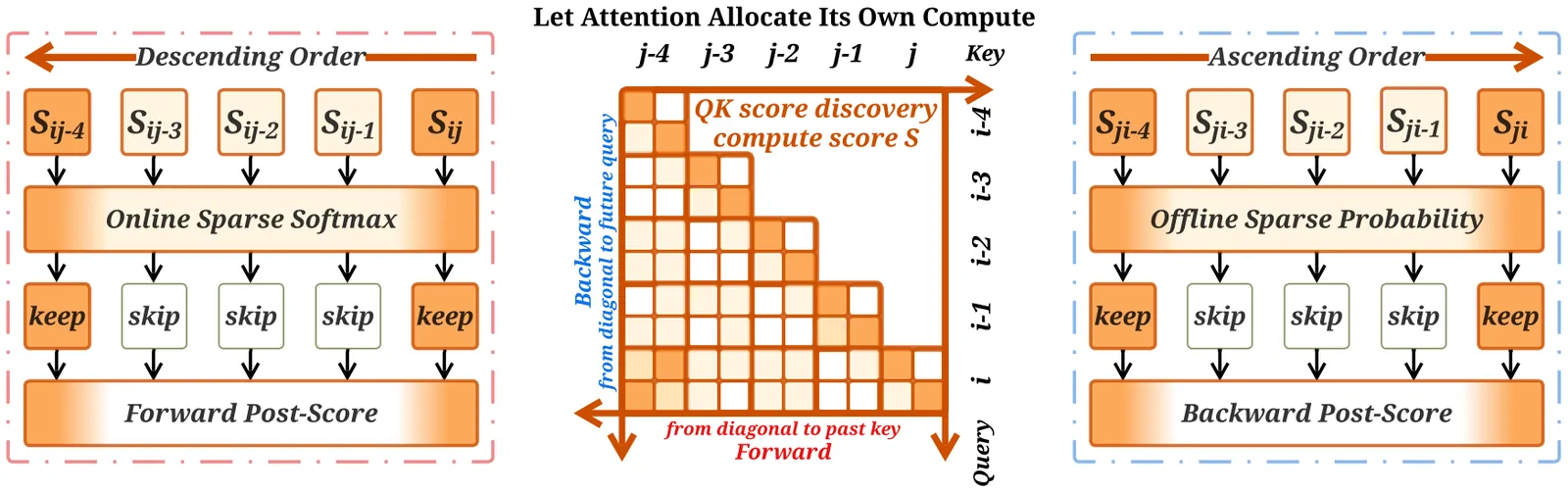
Original Figure 1(fig:teaser). From left to right, it shows the forward and backward flows. Forward uses an evolving online softmax normalizer, while backward reuses the finalized normalizer saved by forward. The key point is that score discovery is retained for all tiles (source: §1, Fig. 1).
Background: The problem they solved
Context lengths are expanding from thousands to hundreds of thousands of tokens. Long-document understanding, multi-turn reasoning, and repository-level code generation are driving this (source: §1). Attention over long contexts substantially increases computation and memory traffic.
FlashAttention greatly improved the IO efficiency of self-attention through tiling, fusion, and online softmax. But that improvement does not change the execution pattern itself. Every legal causal tile still performs all post-score computation once QK scores are produced (source: §1).
The structural limitations of prior methods identified in this paper fall into three broad categories (source: §1, §4).
- Fixed sparse — uses support determined by position, such as local windows, structured blocks, and global tokens. Because it is position-based, it can misalign with the interactions the data actually needs.
- Dynamic sparse — selects tokens/blocks via content-based scores and routing. These can skip the QK computation for excluded interactions entirely, but require separate router, indexer, and mask state for selection.
- Adaptive top-p — chooses support adaptively against an estimated mass target. It estimates mass, and in some cases requires separate threshold calibration.
The gap between them is where MALA sits. What if post-score computation were allocated inside the attention loop according to attention’s own normalized contribution? Preserve QK score access (cut only post-score) and build an efficient fused primitive for both training and inference. This is the research gap the paper explicitly addresses (source: §1, §2.4).
New approach: MassAlloc Attention
MALA reframes sparse attention as “distribution-conditioned compute allocation.” It summarizes three contributions (source: §1).
- Formulation — keep every causal interaction score-accessible, and establish the view that the probability distribution produced by attention determines post-score work (§1).
- Implementation — a fused primitive that pairs an online forward rule with an offline backward rule and uses a common normalized-mass tolerance. It uses only standard attention state; forward has an omitted-mass upper bound, and backward has support nested within the forward support (§2.2, §2.4).
- Evaluation — six-stage validation: matched-work controlled experiments, operator fidelity, controlled associative recall, kernel execution, scaling-law training, and model-level evaluation (§3).
The core design has three points.
One tolerance governs everything
Define a common dimensionless tolerance $\tau$. Relative to the probability $1/L_q$ that uniform attention assigns to each key ($L_q$ is the number of causal keys query $q$ can see), form the length-aware threshold $\tau/L_q$. If a tile’s maximum contribution ratio is below this threshold, the tile is omitted (source: §2.1).
This single $\tau$ governs training forward, training backward, inference prefill, and autoregressive decoding. Across the experiments, the standard value $\tau=1$ is used (source: §3, §2.4). Because the threshold represents an allowed contribution, not a budget, sharp attention rows discard many tiles while diffuse rows keep more.
Forward: online sparse softmax
Forward maintains the running maximum $\mathbf{m}_i$ and shifted normalizer sum $\ell_i$ of standard online softmax. The normalizer over the keys retained so far is
$$ Z_q^{(t)} = \sum_{k \in R_q^{(t)}} \exp(s_{qk}) = \exp\bigl(m_q^{(t)}\bigr)\,\ell_q^{(t)} $$and the maximum contribution ratio of a candidate tile is upper-bounded by
$$ r_{qj}^{(t)} = \frac{\exp\bigl(\max_{k \in J_j \cap \mathcal{C}_q} s_{qk}\bigr)}{Z_q^{(t)}} $$Because the denominator includes only the “mass retained so far”, this ratio can exceed 1, and it upper-bounds the dense-softmax probability of that tile. Taking logs yields the block-level test the kernel actually uses (source: §2.2):
$$ \operatorname{rowmax}(\mathbf{S}_{ij}) - \mathbf{m}_i - \log \ell_i < \log\!\bigl(\tau / \mathbf{L}_i\bigr) $$Omitted tiles leave $\mathbf{m}_i$, $\ell_i$, and the output accumulator $\mathbf{O}_i$ unchanged; only retained tiles perform the standard online-softmax update. The final output is therefore the same as ordinary softmax attention renormalized over the retained tiles (source: §2.2).
Backward: offline sparse probabilities
Backward does not replay the sequence of partial normalizers from forward; it uses the final normalizer $Z_{R,q}$ saved by forward. Here “offline” means the normalizer is already finalized when tiles are examined, not that offline calibration is performed (source: §2.2).
In exact arithmetic, $Z_{R,q} \ge Z_q^{(t)}$, so using the final denominator cannot increase any key’s contribution ratio. Therefore, any tile omitted by forward is necessarily omitted by backward, and backward can additionally omit tiles that forward had retained while the normalizer was still incomplete. As a result, the backward support is nested within the forward support, achieved without storing a forward mask (source: §2.2).
An important nuance: this nesting does not guarantee the exact derivative of the forward operator. Backward may omit additional gradient contributions, and that error also depends on $\mathrm{d}O$ and $V$. Gradient fidelity is therefore measured directly at the operator level (source: §2.2).
Theoretical upper bound on forward omitted mass
Proposition 1 in the appendix provides a quantitative guarantee of how safe forward is. For a query, let $Z_R$ be retained mass and $Z_O$ omitted mass; then the omitted probability mass is bounded by
$$ \epsilon_q = \frac{Z_O}{Z_R + Z_O} \le \frac{\tau}{1+\tau} $$With $\tau=1$, omitted mass can be as high as $50\%$ (a very loose bound), but measured values are orders of magnitude lower (source: Appendix §A.2, Prop. 1). Also, if the norm of value vectors is at most $V_{\max}$, output error is bounded by $\lVert o - \widetilde{o}\rVert \le \frac{2\tau}{1+\tau} V_{\max}$. This assumes exact arithmetic; in the finite precision of a fused implementation, rounding error must also be accounted for (source: Appendix §A.2).
How it works: a concrete example
Let’s trace the abstract decision rule on a small input. (An illustrative example — unrelated to the paper’s experiments; it only demonstrates the mechanism.)
Suppose a single query sees four causal keys (positions $k_0, k_1, k_2, k_3$). Since $\tau=1$, the threshold is $\tau/L_q = 1/4 = 0.25$. Suppose $\exp(\text{score})$ for each key is as follows.
| Key | $\exp(s_k)$ | Meaning |
|---|---|---|
| $k_3$ (most recent) | $e^2 \approx 7.39$ | Recent token of medium strength |
| $k_2$ | $1$ | Weak token |
| $k_1$ (distant) | $e^3 \approx 20.1$ | Strong long-range token |
| $k_0$ | $1$ | Weak token |
Forward traverses from the diagonal ($k_3$) toward the past. Tracking state changes step by step:
| Step | Tile | $Z_q^{(t)}$ | $r_{qj}^{(t)} = \frac{\exp(s)}{Z_q^{(t)}}$ | Decision |
|---|---|---|---|---|
| 1 | $k_3$ | 0 (first tile) | $\infty$ | keep (the first legal tile is always retained) |
| 2 | $k_2$ | 7.39 | $1/7.39 \approx 0.135$ | omit ($0.135 < 0.25$) |
| 3 | $k_1$ | 7.39 | $20.1/7.39 \approx 2.72$ | keep ($2.72 > 0.25$) |
| 4 | $k_0$ | 27.49 | $1/27.49 \approx 0.036$ | omit ($0.036 < 0.25$) |
The final retained set is $\{k_3, k_1\}$, and the output is softmax renormalized over these two. Dense softmax would have given $k_0$ and $k_2$ about $3.4\%$ mass each, but MALA omits them. Two points matter. (1) Both the recent token ($k_3$) and the strong long-range token ($k_1$) are retained — locality is only a prior on execution order, not a support assumption. (2) Weak tokens fall below the threshold and are omitted.
In this 4-token example, omitted mass looks large at about $6.8\%$, but at realistic large-context scales $L_q$ is in the thousands to tens of thousands, so $\tau/L_q$ becomes extremely small and mass concentrates on a few tokens; the omitted mass reported in the paper falls to around $0.006\%$ (source: §3, Fig. 2). This example only shows which decisions occur in what order.
The same decision process repeats in backward, but backward uses the final normalizer ($27.49$) directly and can therefore be more selective than forward. For example, if forward retained a tile (at an early stage when the normalizer was still small), backward can omit it additionally (source: §2.2).
Performance validation: main results
The authors validate in six stages that ask progressively broader questions: allocation quality at fixed work → fidelity across context lengths → long-range association → kernel execution efficiency → quality-cost across model scales → full model evaluation (source: §3).
1) With equal work, allocation is decisive
The most compelling experiment is the “matched-work” control. At 8K context, all policies perform exactly the same total post-score work (about 1,024 slots per query), and only how the work is distributed is compared (source: §3, Table 1).
| Allocation scope | Selection signal | Mean omitted mass | Mean output error |
|---|---|---|---|
| Position only (position) | Final reference mass | 0.6012% | 0.6231% |
| Layer/head/position | Final reference mass | 0.1721% | 0.2817% |
| Input/layer/head/position (per-instance oracle) | Final reference mass | 0.0182% | 0.0164% |
| MALA (online mass upper bound) | Online mass | 0.0188% | 0.0174% |
Moving from static allocation to per-input allocation (oracle) cuts omitted mass by $9.5\times$ and output error by $17.2\times$. MALA’s online test nearly matches this oracle (0.0188% vs. 0.0182%). In other words, the source of the gain is not “work” but “distribution-adaptive allocation” itself (source: §3, Table 1).
2) One tolerance holds across contexts
Running 1K–32K-token prefixes with the same $\tau=1$, forward work increases from 470 to 1,066 slots per query and backward from 462 to 1,058, then stabilizes at 1,010–1,066 after 8K. This stable range is why the experiments below use a reference of “about 1,024 slots.” Across all lengths, omitted mass is at most 0.0062% (P95 0.032%) and relative output error at most 0.021% (P95 0.14%). Gradient errors are within 0.38% for $\mathrm{d}Q$, 0.35% for $\mathrm{d}K$, and 0.17% for $\mathrm{d}V$ (source: §3, Fig. 2).
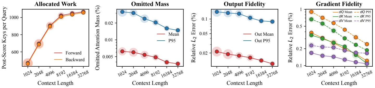
Original Figure 2(fig:operator_fidelity). The horizontal axis is context length (1K–32K); the top panel is mean post-score key slots per query; the bottom panel is relative error for omitted mass, output, and gradients. Even as context grows $32\times$, work flattens after 8K and error stays low — evidence for the claim that a single tolerance covers all lengths (source: §3, Fig. 2).
3) Long-range association is preserved
On controlled associative recall (256 key-value pairs), MALA tracks FullAttn closely as context grows. At sequence length 8,192 and $d_{model}=512$, MALA scores 89.67% vs. FullAttn 89.97%, while fixed-budget sparse methods collapse — DSA 52.61%, MoBA 47.25%, NSA 22.61% (source: §3, Fig. 3).
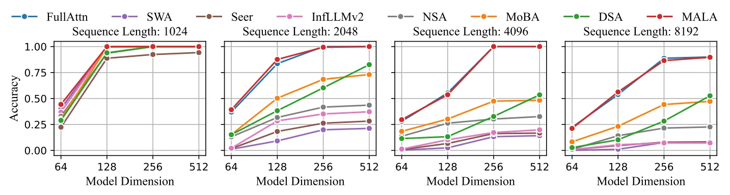
Original Figure 3(fig:ar). Panels are model dimensions ($d_{model}$=64–512); curves are accuracy versus sequence length (1,024–8,192). MALA stays close to the FullAttn curve, whereas fixed-budget (1,024 slots) sparse methods lose associations substantially as context grows. This supports the central claim that “support allocated by attention itself preserves associations that external selection or fixed support miss” (source: §3, Fig. 3).
4) Latency drops in real kernels
Measured on 8 H100 GPUs with tensor parallelism $TP=8$ at 128K tokens. MALA reduces training forward latency by $2.2\times$, backward by $3.0\times$, and inference decoding by $1.6\times$ versus FullAttn. It has the lowest forward/backward latency among the compared methods, and its decoding is within 3% of DSA while being $1.6\times$ faster than FullAttn. Because allocation is fused into the attention loop and uses only standard attention state, peak memory remains at FullAttn’s level (source: §3, Fig. 4).
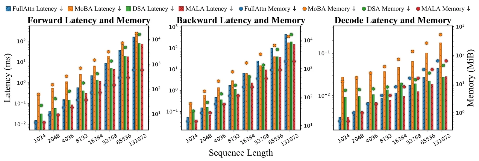
Original Figure 4(fig:latency_memory). The three panels show latency (left axis, bars) and per-rank peak memory (right axis, markers) for forward, backward, and decoding, respectively. FullAttn/MoBA/DSA/MALA are compared; MALA lowers latency while keeping peak memory at the same level as FullAttn. Measurements include the entire score-discovery and selection path of each method (source: §3, Fig. 4).
5) The quality-cost frontier shifts toward lower FLOPs
In scaling-law training at five scales from 0.6B to 14B, MALA tracks FullAttn’s perplexity closely while reducing total training FLOPs. At 14B, the perplexity difference is below 0.001 in both stages, while total FLOPs are reduced by $2.5\%$ in 4K pretraining and $23.1\%$ in 32K long-context training. The larger saving in long context occurs because MALA performs only the post-score work justified by the realized distribution while still including the full causal QK score-discovery cost (source: §3, Fig. 5).
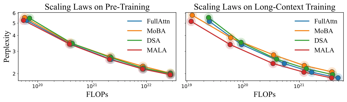
Original Figure 5(fig:scaling_laws_flops). The left panel is the perplexity–FLOPs curve for 4K pretraining and the right for 32K long-context training. The FLOPs axis includes full score discovery and each method’s allocation/selection cost. The key point is that the MALA curve shifts left (lower cost) while tracking FullAttn closely — the gap widens especially in the 32K panel (source: §3, Fig. 5).
6) Model-level quality is preserved
Evaluation summary for the final 14B model and for a 32B model trained further in a separate run (source: §3, Table 2).
| Scale | Method | Knowledge | Reasoning | RULER 32K | RULER 128K |
|---|---|---|---|---|---|
| 14B | FullAttn | 72.32 | 64.46 | 89.42 | 65.84 |
| 14B | MoBA | 70.01 | 58.07 | 86.85 | 60.17 |
| 14B | DSA | 70.11 | 62.04 | 87.59 | 63.05 |
| 14B | MALA | 72.48 | 64.66 | 89.45 | 65.75 |
| 32B | FullAttn | 75.62 | 75.67 | 92.70 | 82.03 |
| 32B | MALA | 75.75 | 76.10 | 92.71 | 82.56 |
On average across knowledge, reasoning, 32K base retrieval, and YaRN-extrapolated 128K retrieval, MALA matches or slightly exceeds FullAttn at both scales. Notably, MoBA and DSA with a fixed budget fall substantially behind FullAttn at 14B (knowledge 70.01/70.11, reasoning 58.07/62.04), whereas MALA, which has no fixed budget, is on par with FullAttn (source: §3, Table 2, Appendix Tables 5–7).
Our perspective: strengths, limitations, and why this work matters
Strengths
The paper’s greatest virtue is its experimental design that isolates causality. The matched-work control (Table 1) uses an oracle comparison to show that “the gain comes not from less work but from distribution-adaptive allocation”; operator fidelity (Fig. 2) independently verifies the tolerance’s generality; associative recall (Fig. 3) independently verifies preservation of long-range associations; kernel measurements (Fig. 4) independently verify real speedups; and scaling laws (Fig. 5) independently verify scalability. Each experiment fills a gap left by another.
On the design side it is also clean. A single $\tau$ spans training and inference, no separate mask, index, or router state is created, and forward omitted mass has an explicit upper bound (Prop. 1). The property that backward support is nested within forward support ensures consistency between the two passes without storage overhead (source: §2.4, Appendix §A.2).
Limitations
Start with the limitations the authors explicitly acknowledge.
- QK complexity remains quadratic. The saving is only a data-dependent constant-factor reduction in post-score computation; score discovery is still performed in full (source: §2.3, §5). Support-sparse methods are complementary to MALA in that they can skip QK computation for excluded regions entirely.
- Backward is not the exact derivative of forward. Nesting does not guarantee an approximate derivative, so gradient fidelity is verified by measurement rather than theory (source: §2.2).
- The bound in Prop. 1 assumes exact arithmetic; in the finite precision of a fused implementation, rounding error is added (source: Appendix §A.2).
As a reviewer, I would note the following potential limitations.
- The sensitivity of $\tau=1$ was not validated. The claim is that a common tolerance works universally without separate calibration, but the main text has no ablation varying $\tau$. Unlike families such as Top-Theta that perform offline calibration, the optimality of insisting on a single constant remains open (source: §4).
- Absolute latency and cost are not reported. Only relative factors such as $2.2\times$/$3.0\times$/$1.6\times$ are given; there is no latency in ms or cost in dollars per 1M tokens. Actual savings depend on context length, distribution, and batch size, so absolute values under operating conditions are unverified (source: §3).
- The decoding saving ($1.6\times$) is smaller than the training savings ($2.2\times$/$3.0\times$). This appears to be because QK score discovery accounts for a larger share during single-token decoding. The benefit in latency-sensitive serving environments may not be as pronounced as in training.
- It does not touch the KV cache itself. MALA neither compresses nor evicts the cache; it keeps it intact, so savings in cache-capacity-bound scenarios are left to separate techniques (source: §2.4, §4).
Why this work matters
Whereas prior efficient-attention work has mostly focused on which tokens/blocks to look at (support selection), MALA opens a complementary axis: look at all the scores, but choose which work to do afterward. These two axes are not mutually exclusive. Combining support sparsity, which reduces score discovery, with MALA, which reduces post-score work, could optimally reduce QK computation and post-score computation separately. In particular, the result that “FullAttn quality is maintained without a fixed budget” shows a way around the long-standing pain of tuning the budget hyperparameter in sparse attention (source: §1, §4).
What’s next?: The road ahead
The authors do not provide an explicit future-work list in the conclusion. Instead, in the related-work section they state that MALA “retains the full KV history for score discovery and value access, leaving cache storage and placement as separate optimization opportunities” (source: §4, §5). Combining this direction with the limitations above suggests the following reasonable next steps.
- Reduce QK discovery too — combine with support-sparse methods (MoBA, DSA, etc.). Reducing the quadratic cost of score discovery while preserving post-score savings is the next bottleneck for long-context scalability.
- Automatic/offline calibration of $\tau$ — go beyond validating a single constant’s generality and measure the quality-cost Pareto frontier when $\tau$ is calibrated per layer, head, and context length.
- Validate absolute serving metrics — report absolute decoding latency (ms/token), TTFT, and batch scalability to confirm benefits from an operational rather than training-centric perspective.
- Longer contexts (1M+) and other modalities — YaRN 128K extrapolation has already been verified, but test whether the same normalized-mass allocation holds for native ultra-long contexts and vision/multimodal attention.
- Combine with KV cache management — add compression/eviction techniques on top of the full KV cache that MALA retains, covering cache-capacity-bound scenarios as well.
The idea of letting attention allocate its own computation is simple, but it is presented with a cumulative six-stage experimental design, symmetric forward/backward rules, and a theoretical upper bound, making it highly convincing. The source is available at HKUSTDial/flash-sparse-attention (source: Abstract).
Tables from the paper
Tables converted mechanically from the arXiv e-print LaTeX source. The numbers are the paper’s own and did not pass through a model.
Table 1. Matched-work allocation. Every policy executes exactly the same total post-score work, with a shared average of approximately 1,024 slots per query. The first three rows use finalized per-instance reference mass for region selection and differ only in how work is allocated across decisions. Omitted probability mass and relative output $L_2$ error are reported as percentages; statistics pool input-layer-head-query-block allocation decisions.
| Allocation Scope | Selection Signal | Mean Slots | Omitted Mass (%) Mean $\downarrow$ | Omitted Mass (%) P95 $\downarrow$ | Output Error (%) Mean $\downarrow$ | Output Error (%) P95 $\downarrow$ |
|---|---|---|---|---|---|---|
| Position | Final reference mass | $\approx$1,024 | $0.6012$ | $0.9923$ | $0.6231$ | $4.237\phantom {0}$ |
| Layer/Head/Position | Final reference mass | $\approx$1,024 | $0.1721$ | $0.6247$ | $0.2817$ | $0.9237$ |
| Input/Layer/Head/Position | Final reference mass | $\approx$1,024 | $\mathbf{0.0182}$ | $\mathbf{0.0664}$ | $\mathbf{0.0164}$ | $\mathbf{0.1013}$ |
| Input/Layer/Head/Position | MALA online mass bound | $\approx$1,024 | $\underline{0.0188}$ | $\underline{0.0693}$ | $\underline{0.0174}$ | $\underline{0.1017}$ |
Table 2. Model-level evaluation summary. Average knowledge and reasoning scores, together with RULER scores at the native 32K context length and after YaRN extrapolation to 128K. Detailed per-task results and uncertainty estimates are reported in Appendix .
| Model Scale | Method | Knowledge | Reasoning | RULER 32K | RULER 128K |
|---|---|---|---|---|---|
| 14B | FullAttn | 72.32 | 64.46 | 89.42 | 65.84 |
| 14B | MoBA | 70.01 | 58.07 | 86.85 | 60.17 |
| 14B | DSA | 70.11 | 62.04 | 87.59 | 63.05 |
| 14B | MALA (ours) | 72.48 | 64.66 | 89.45 | 65.75 |
| 32B | FullAttn | 75.62 | 75.67 | 92.70 | 82.03 |
| 32B | MALA (ours) | 75.75 | 76.10 | 92.71 | 82.56 |
Table 3. Associative-recall allocation configurations. Fixed-budget sparse methods use a common 1,024-slot ceiling, with realized work computed after causal clipping and native block expansion. The raw-slot comparison aligns retained interactions; DSA therefore uses the same slot ceiling despite its larger value dimension. MALA uses $\tau=1$, with work determined by normalized-mass allocation.
| Method | Allocation Rule | $d_v/d_{v,\mathrm{ref}}$ | Nominal Slot Ceiling | Raw-Slot Reference |
|---|---|---|---|---|
| FullAttn | Complete causal history | $1\times$ | Full | Full |
| SWA / Seer / InfLLMv2 / NSA | Native support or selector | $1\times$ | 1,024 | after causal clipping |
| MoBA | Native block routing | $1\times$ | 1,024 | after causal clipping |
| DSA | Token-level Top-$K$ | $4\times$ | 1,024 | after causal clipping |
| MALA | Normalized-mass tolerance $\tau=1$ | $1\times$ | - | measured near reference |
Table 4. Operator benchmark configurations. The sparse methods target comparable forward post-score FLOP-equivalent work, while reported latency and memory include their complete score-discovery and selection paths.
| Method | $n_h$ | $n_{h_{kv}}$ | $d_{qk}$ | $d_v$ | Allocation | Target Eq. Slots | Precision |
|---|---|---|---|---|---|---|---|
| FullAttn\footnotemark[1] | 64 | 8 | 128 | 128 | Full causal context | Full | BF16 |
| MoBA\footnotemark[2] | 64 | 64 | 128 | 128 | $B=128$, native routing | $\approx$1,024 | BF16 |
| DSA\footnotemark[3],\footnotemark[4] | 64 | 1 | 576 | 512 | Top-$K=256$, FP8 indexer | $\approx$1,024 | BF16/FP8 |
| MALA | 64 | 8 | 128 | 128 | $\tau=1$, fused allocation | measured $\approx$1,024 | BF16 |
Table 5. Self-Attention Variants Scaling Laws Configurations. Complete model, training, and attention configurations used in the scaling-law experiments. PS FLOPs/Slot describes allocated forward post-score work; the FLOP-axis additionally includes complete score discovery and method-specific selection.
| Algos | Params | PT/LCT Tok | Batch | PT/LCT LR | $n_{layers}$ | $d_{model}$ | $n_h$ | $n_{h_{kv}}$ | $d_{qk}$ | $d_v$ | PS FLOPs/Slot | PT Alloc | LCT Alloc |
|---|---|---|---|---|---|---|---|---|---|---|---|---|---|
| FullAttn | $\approx$0.6B | 12B,1.5B | 0.256M | 1e-3,1e-4 | 28 | 1024 | 16 | 8 | 128 | 128 | 4096 | 4096 | 32768 |
| MoBA | $\approx$0.6B | 12B,1.5B | 0.256M | 1e-3,1e-4 | 28 | 1024 | 16 | 16 | 128 | 128 | 4096 | $K=1024$ | $K=1024$ |
| DSA | $\approx$0.6B | 12B,1.5B | 0.256M | 1e-3,1e-4 | 28 | 1024 | 16 | 1 | 576 | 512 | 16384 | $K=256$ | $K=256$ |
| MALA | $\approx$0.6B | 12B,1.5B | 0.256M | 1e-3,1e-4 | 28 | 1024 | 16 | 8 | 128 | 128 | 4096 | $\tau=1$ | $\tau=1$ |
| FullAttn | $\approx$1.7B | 34B,4B | 0.512M | 8e-4,8e-5 | 28 | 2048 | 16 | 8 | 128 | 128 | 4096 | 4096 | 32768 |
| MoBA | $\approx$1.7B | 34B,4B | 0.512M | 8e-4,8e-5 | 28 | 2048 | 16 | 16 | 128 | 128 | 4096 | $K=1024$ | $K=1024$ |
| DSA | $\approx$1.7B | 34B,4B | 0.512M | 8e-4,8e-5 | 28 | 2048 | 16 | 1 | 576 | 512 | 16384 | $K=256$ | $K=256$ |
| MALA | $\approx$1.7B | 34B,4B | 0.512M | 8e-4,8e-5 | 28 | 2048 | 16 | 8 | 128 | 128 | 4096 | $\tau=1$ | $\tau=1$ |
| FullAttn | $\approx$4B | 80B,10B | 1M | 6e-4,6e-5 | 32 | 2560 | 32 | 8 | 128 | 128 | 8192 | 4096 | 32768 |
| MoBA | $\approx$4B | 80B,10B | 1M | 6e-4,6e-5 | 32 | 2560 | 32 | 32 | 128 | 128 | 8192 | $K=1024$ | $K=1024$ |
| DSA | $\approx$4B | 80B,10B | 1M | 6e-4,6e-5 | 32 | 2560 | 32 | 1 | 576 | 512 | 32768 | $K=256$ | $K=256$ |
| MALA | $\approx$4B | 80B,10B | 1M | 6e-4,6e-5 | 32 | 2560 | 32 | 8 | 128 | 128 | 8192 | $\tau=1$ | $\tau=1$ |
| FullAttn | $\approx$8B | 164B,20B | 1.6M | 4e-4,4e-5 | 36 | 4096 | 32 | 8 | 128 | 128 | 8192 | 4096 | 32768 |
| MoBA | $\approx$8B | 164B,20B | 1.6M | 4e-4,4e-5 | 36 | 4096 | 32 | 32 | 128 | 128 | 8192 | $K=1024$ | $K=1024$ |
| DSA | $\approx$8B | 164B,20B | 1.6M | 4e-4,4e-5 | 36 | 4096 | 32 | 1 | 576 | 512 | 32768 | $K=256$ | $K=256$ |
| MALA | $\approx$8B | 164B,20B | 1.6M | 4e-4,4e-5 | 36 | 4096 | 32 | 8 | 128 | 128 | 8192 | $\tau=1$ | $\tau=1$ |
| FullAttn | $\approx$14B | 296B,36B | 2M | 3e-4,3e-5 | 40 | 5120 | 40 | 8 | 128 | 128 | 10240 | 4096 | 32768 |
| MoBA | $\approx$14B | 296B,36B | 2M | 3e-4,3e-5 | 40 | 5120 | 40 | 40 | 128 | 128 | 10240 | $K=1024$ | $K=1024$ |
| DSA | $\approx$14B | 296B,36B | 2M | 3e-4,3e-5 | 40 | 5120 | 40 | 1 | 576 | 512 | 40960 | $K=256$ | $K=256$ |
| MALA | $\approx$14B | 296B,36B | 2M | 3e-4,3e-5 | 40 | 5120 | 40 | 8 | 128 | 128 | 10240 | $\tau=1$ | $\tau=1$ |
Table 6. Knowledge Benchmark Results. Knowledge evaluation of the scaling-law models at 14B and the continued-training models at 32B. MALA produces averages comparable to FullAttn at both scales and remains close across individual tasks.
| Model | MMLU | MMLU-Pro | BBH | HellaSwag | OBQA | WinoGrande | Avg |
|---|---|---|---|---|---|---|---|
| Gen|5-shot | 5-shot | CoT|3-shot | 5-shot | 5-shot | 5-shot | ||
| 14B-Non-Thinking, temperature=0.6, top_k=20, top_p=0.95, max_gen_toks=32768, seed=[0, 42, 233, 666, 1234] | |||||||
| FullAttn | 78.21$\pm$0.31 | 64.96$\pm$0.46 | 82.59$\pm$0.48 | 80.64$\pm$0.38 | 49.4$\pm2.17$ | 78.16$\pm$1.14 | 72.32 |
| MoBA | 75.78$\pm$0.48 | 58.42$\pm$0.84 | 82.1$\pm$0.44 | 79.7$\pm$0.37 | 49.49$\pm$2.07 | 74.57$\pm$1.47 | 70.01 |
| DSA | 72.5$\pm$0.53 | 59.56$\pm$0.65 | 81.42$\pm$0.62 | 80.22$\pm$0.31 | 49.41$\pm$2.25 | 77.57$\pm$1.19 | 70.11 |
| MALA (ours) | 78.14$\pm$0.31 | 64.67$\pm$0.44 | 82.54$\pm$0.48 | 80.61$\pm$0.36 | 50.0$\pm$2.17 | 78.93$\pm$1.13 | 72.48 |
| 32B-Thinking, temperature=0.6, top_k=20, top_p=0.95, max_gen_toks=32768, seed=[0, 42, 233, 666, 1234] | |||||||
| FullAttn | 77.27$\pm$0.34 | 68.57$\pm$0.41 | 88.39$\pm$0.54 | 83.4$\pm$0.37 | 55.0$\pm$2.23 | 81.14$\pm$1.1 | 75.62 |
| MALA (ours) | 77.37$\pm$0.33 | 68.33$\pm$0.41 | 88.23$\pm$0.55 | 84.69$\pm$0.36 | 55.0$\pm$2.23 | 80.87$\pm$1.13 | 75.75 |
Table 7. Reasoning Benchmark Results. Reasoning evaluation of the scaling-law models at 14B and the continued-training models at 32B. MALA matches FullAttn on average at 14B and 32B without a fixed retained-work budget.
| Model | PIQA | GSM8K | Hendrycks-Math | ARC-C | AGIEval | GPQA-Diamond | Avg |
|---|---|---|---|---|---|---|---|
| 5-shot | CoT|4-shot | CoT|4-shot | 0-shot | 0-shot | CoT|3-shot | ||
| 14B-Non-Thinking, temperature=0.6, top_k=20, top_p=0.95, max_gen_toks=32768, seed=[0, 42, 233, 666, 1234] | |||||||
| FullAttn | 81.63$\pm$0.86 | 90.32$\pm$0.93 | 62.46$\pm$0.65 | 61.95$\pm$1.44 | 50.56$\pm$0.71 | 39.87$\pm$3.47 | 64.46 |
| MoBA | 77.54$\pm$0.94 | 87.53$\pm$1.02 | 38.67$\pm$1.39 | 61.35$\pm$0.63 | 46.5$\pm$0.81 | 36.87$\pm$3.52 | 58.07 |
| DSA | 80.35$\pm$0.82 | 89.38$\pm$0.95 | 53.24$\pm$0.86 | 61.74$\pm$1.33 | 47.0$\pm$0.69 | 40.53$\pm$3.86 | 62.04 |
| MALA (ours) | 81.62$\pm$0.85 | 90.83$\pm$0.9 | 62.34$\pm$0.64 | 61.93$\pm$1.47 | 50.54$\pm$0.71 | 40.67$\pm$3.32 | 64.66 |
| 32B-Thinking, temperature=0.6, top_k=20, top_p=0.95, max_gen_toks=32768, seed=[0, 42, 233, 666, 1234] | |||||||
| FullAttn | 85.97$\pm$0.88 | 93.33$\pm$0.69 | 94.94$\pm$0.82 | 69.54$\pm$1.34 | 54.18$\pm$0.68 | 56.06$\pm$3.54 | 75.67 |
| MALA (ours) | 85.94$\pm$0.88 | 95.45$\pm$0.57 | 94.25$\pm$0.83 | 69.8$\pm$1.34 | 53.87$\pm$0.66 | 57.29$\pm$2.89 | 76.1 |
Table 8. Retrieval Benchmark Results. RULER evaluation at the native 32K context length and after YaRN extrapolation to 128K. MALA remains comparable to FullAttn across both model scales and context lengths.
| Model | NIAH-S | NIAH-MK | NIAH-MQ | NIAH-MV | RULER-VT | RULER-CWE | RULER-FWE | RULER-QA | Avg |
|---|---|---|---|---|---|---|---|---|---|
| 14B Native 32K Sequence Length, seed=[0, 42, 233, 666, 1234] | |||||||||
| FullAttn | 100$\pm$0 | 98.0$\pm$0.65 | 98.8$\pm$0.68 | 95.5$\pm$0.72 | 99.44$\pm$0.2 | 75.7$\pm$0.69 | 91.67$\pm$0.71 | 56.28$\pm$1.2 | 89.42 |
| MoBA | 99.2$\pm$0.4 | 93.2$\pm$0.66 | 98.3$\pm$0.71 | 94.8$\pm$0.73 | 99.08$\pm$0.33 | 66.8$\pm$0.99 | 91.3$\pm$0.72 | 52.02$\pm$1.64 | 86.85 |
| DSA | 99.8$\pm$0.2 | 95.2$\pm$0.69 | 97.8$\pm$0.79 | 95.4$\pm$0.74 | 98.87$\pm$0.31 | 69.05$\pm$0.89 | 91.1$\pm$0.74 | 53.51$\pm$1.52 | 87.59 |
| MALA (ours) | 100$\pm$0 | 97.5$\pm$0.68 | 98.6$\pm$0.68 | 95.3$\pm$0.73 | 99.03$\pm$0.22 | 74.32$\pm$0.74 | 93.76$\pm$0.59 | 57.05$\pm$1.18 | 89.45 |
| 32B Native 32K Sequence Length, seed=[0, 42, 233, 666, 1234] | |||||||||
| FullAttn | 100$\pm$0 | 99.87$\pm$0.09 | 99.8$\pm$0.08 | 99.4$\pm$0.13 | 99.64$\pm$0.18 | 85.18$\pm$0.51 | 94.53$\pm$0.53 | 63.2$\pm$0.93 | 92.7 |
| MALA (ours) | 100$\pm$0 | 99.53$\pm$0.11 | 99.95$\pm$0.05 | 99.25$\pm$0.19 | 99.88$\pm$0.07 | 83.3$\pm$0.54 | 96.33$\pm$0.81 | 63.44$\pm$1.02 | 92.71 |
| 14B YaRN 128K Sequence Length, seed=[0, 42, 233, 666, 1234] | |||||||||
| FullAttn | 98.4$\pm$0.51 | 55.2$\pm$1.64 | 88.25$\pm$0.69 | 64.1$\pm$1.16 | 93.04$\pm$0.63 | 5.76$\pm$0.46 | 84.26$\pm$0.79 | 37.73$\pm$2.15 | 65.84 |
| MoBA | 92.2$\pm$0.83 | 51.6$\pm$1.85 | 80.3$\pm$0.87 | 62.05$\pm$1.3 | 90.48$\pm$0.71 | 0.02$\pm$0.06 | 79.93$\pm$0.95 | 24.78$\pm$2.63 | 60.17 |
| DSA | 96.4$\pm$0.62 | 52.7$\pm$1.73 | 83.6$\pm$0.81 | 64.3$\pm$1.16 | 92.48$\pm$0.62 | 4.8$\pm$0.52 | 77.93$\pm$1.16 | 32.19$\pm$2.03 | 63.05 |
| MALA (ours) | 98.6$\pm$0.53 | 54.6$\pm$1.67 | 88.2$\pm$0.69 | 64.2$\pm$1.14 | 93.08$\pm$0.63 | 5.51$\pm$0.45 | 84.17$\pm$0.81 | 37.62$\pm$2.12 | 65.75 |
| 32B YaRN 128K Sequence Length, seed=[0, 42, 233, 666, 1234] | |||||||||
| FullAttn | 99.8$\pm$0.12 | 86.4$\pm$1.35 | 95.7$\pm$0.56 | 88.0$\pm$0.79 | 98.76$\pm$0.22 | 45.68$\pm$1.03 | 93.27$\pm$1.25 | 48.61$\pm$2.17 | 82.03 |
| MALA (ours) | 99.65$\pm$0.13 | 86.3$\pm$1.35 | 95.9$\pm$0.66 | 87.75$\pm$0.79 | 98.69$\pm$0.23 | 45.8$\pm$1.04 | 96.33$\pm$0.81 | 50.03$\pm$1.97 | 82.56 |
Figures in this post are taken from the original arXiv:2609.32712 (CC BY 4.0). Only size and format were changed.
Comments