Flash-dLLM: I/O-First Diffusion LLM Acceleration, Unlocking 210.6 tokens/s with Fused Cache and Self-Verification
One-Line Summary (TL;DR)
Diffusion LLMs (dLLMs) support parallel denoising, but combining KV cache reuse with parallel decoding makes GPU memory I/O the bottleneck (source: §1). Flash-dLLM combines Flash-Cache, which fuses QKV projection, RoPE, and cache writes in SRAM with no training, and Flash-Verify, in which the dLLM itself serves as both drafter and verifier, achieving 210.6 tokens/s on GSM8K-512 with LLaDA-1.5, an 81.0× speedup, and 5.1× and 11.0× speedups over Elastic-Cache (source: Tab. 1, Tab. 2, Abstract).
Core Ideas
- I/O is the real bottleneck: caching reduces FLOPs but repeats HBM reads/writes four times (source: §2.2, Fig. 1a). The fix is to reduce movement, not computation.
- No need to see everything: in middle layers, the top 32 tokens account for about 50% of total attention (source: Fig. 1b). Track only a fixed budget $\beta_t$ and serve the rest from cache.
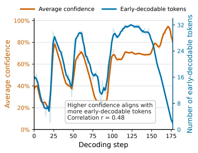
- Confidence is throughput: mean confidence and the number of early-decodable tokens show a positive correlation of $r=0.48$ (source: Fig. 1c). Self-verifying discarded low-confidence predictions with two views doubles tokens per step (source: Fig. 6).
Background: The Problem They Solved
Research Gap
dLLMs do not generate left-to-right but refine a masked sequence over multiple passes (source: §1). This paradigm has been extended to LLaDA, Dream, Gemini Diffusion, and Mercury, but open-source dLLM inference has lagged behind autoregressive LLM optimizations for KV caching, attention kernels, and speculative decoding (source: §1, §4).
At publication time, the state of the art had three branches (source: §2.1, §4):
- Fast-dLLM: prefix caching and confidence-based parallel decoding. It unmasks in one shot only tokens whose confidence $c_i$ exceeds a threshold $\epsilon$.
- Elastic-Cache: adaptive cache reuse based on attention pattern drift. It is the baseline inheriting sliding-window decoding (source: §2.1).
- dKV-Cache, dllm-Cache, Dyna-dLLM, FreeDave, FlashDLM: fixed-interval caching, adaptive caching, external autoregressive verifiers, two-pass verification, and others.
The critical limitation is that they treated caching and parallel decoding separately (source: Abstract). In practice, the changing query set $Q_t$ at every step causes frequent cache reads/writes/updates, while uniformly processing tokens that are unchanged or have little influence wastes memory bandwidth (source: §1). Second, they ignored token-level sparsity. Third, they left the mismatch in confidence dynamics unresolved. Many tokens are already semantically determined, but a conservative $\epsilon$ delays commitment and wastes refinement steps (source: §1).
Core Hypothesis
The authors assume that existing caching limits can be overcome and denoising steps can be reduced without quality loss, achieving wall-clock speedup and memory scalability, by removing unnecessary HBM movement with a fused I/O-aware cache, selectively reusing only high-impact decoding tokens, and introducing two-view verification that uses the dLLM itself as drafter and verifier (source: §1-§2.3).
New Approach: Flash-dLLM
Flash-dLLM is a training-free inference framework (source: Abstract). It consists of two modules (source: Fig. 2, Alg. 2).
Flash-Cache: I/O-Aware KV Caching
1. Fused kernel. Existing implementations run QKV projection, RoPE, cache writes, and attention in separate CUDA kernels per layer (source: §2.2). Because each kernel writes to HBM and the next kernel reads it, per-layer traffic is about $4 \times O(Q d_{\text{model}}) + O(N d)$. Flash-Cache takes inspiration from FlashAttention to perform projection and RoPE in SRAM and write keys and values directly to the KV cache (source: Fig. 3a, Alg. 1). It removes intermediate KV materialization and reduces HBM traffic and memory usage.
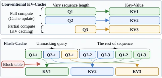
2. Scheduled flash attention. In dLLM batches, the lengths of the caching stage and the full-update stage differ widely across samples (source: §2.2). Instead of padding or forced synchronization, the batch is split into multiple sequence blocks, and a block table aligns query blocks with KV blocks (source: Fig. 3b). It differs from prior FlashAttention in its focus on controlling which blocks to compute and in what order.
3. Selective cache update. The next query is kept at a fixed size (source: §2.2):
$$ Q_{t+1} = M_{t+1}^{\beta_m} \cup T_{t+1} $$where $M_{t+1}^{\beta_m}$ is a masked sliding window of size $\beta_m$ and $T_{t+1}$ is a tracked set of size $\beta_t$. The importance of a decoded token $i$ is measured by how much masked queries attended to it:
$$ a_i^t = \sum_{l=1}^{L} \frac{1}{H} \sum_{h=1}^{H} \frac{1}{|M_t^{\beta_m}|} \sum_{j \in M_t^{\beta_m}} S_{j,i}^{t,l,h}, \quad i \in D_{Flash-Verify: Cache-Based Draft-Verification Parallel Decoding
Conventional confidence-based decoding accepts only tokens with $c_i \ge \epsilon$ and discards the rest (source: §2.3). On uncertain tasks, per-step acceptance hits a ceiling.
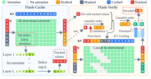
Flash-Verify queries the full KV cache for $Q_t = T_t \cup M_t^{\beta_m}$ in the draft pass and sorts masked positions by confidence into a confident set $D_t$ and an exploratory set $S_t$ (source: Alg. 2). The verification pass builds new queries from three groups: an adjusted tracked set $T_v$, a draft view that fills $S_t$ with draft predictions, and a mask view that fills the same positions with [MASK]. The two views share position embeddings but cannot see each other through a causal mask (source: §2.3, Fig. 2).
The acceptance rule is simple:
$$ \text{accept}(i) = \mathbb{I}[\hat{x}_i = \tilde{x}_i] \cdot \mathbb{I}[\tilde{c}_i \ge \gamma] $$$\hat{x}_i$ is the draft prediction, and $\tilde{x}_i$ and $\tilde{c}_i$ are the mask-view prediction and confidence. It accepts sequentially in decoding order only up to the first mismatch (source: §2.3). The extra cost scales with $2\beta_m$, not the full sequence, and no external model is needed.
There is also a theoretical guarantee (source: Appx. C). Let $p_i$ be the mask-view verification conditional distribution and $\pi_i$ the committed point mass; for each accepted token:
$$ \text{TV}(\pi_i, p_i) = 1 - \tilde{c}_i \le 1 - \gamma $$For a block $A = \{i_1,\dots,i_m\}$, $\text{TV}(\pi_A, p_A) = 1 - \prod_k \tilde{c}_{i_k} \le 1 - \gamma^m \le m(1-\gamma)$. Because the verification mask is causal, $p_A$ is the model’s true joint, not a product of marginals, and verification tokens introduce no parallel-unmasking dependency error (source: Appx. C, Remark 1). Lowering $\epsilon$ is not equivalent to verification, because $\epsilon$ splits the draft marginals in the all-masked state while $\gamma$ splits the distribution that is actually committed (source: Appx. C, Remark 2).
How It Works: A Concrete Example
Consider a mini example for a graduate student. The vocabulary contains only {A, B, [MASK]}, with generation length $N=4$, $\beta_m=2$, $\beta_t=1$, $\epsilon=0.9$, and $\gamma=0.8$ (variable definitions borrowed from §2.2-§2.3).
Let the input be $x_0 =$ [BOS] [MASK] [MASK] [MASK] [MASK], $D_{<1} = \{1\}$, and $M_1 = \{2,3,4,5\}$. Here $Q$ is the query positions, $K$ and $V$ are the cache, $D_t$ is newly decoded positions, $M_t^{\beta_m}$ is the front $\beta_m$ masks, $T_t$ is the tracked set, and $S_t$ is verification targets.
Step 1: Draft. Since $M_1^{\beta_m}=\{2,3\}$ and $T_1=\emptyset$, $Q_1=\{2,3\}$. The fused kernel reads only $x[Q_1]$ to build $q,k,v$ in SRAM and writes them directly to cache (source: Alg. 1). After attending over the full cache, suppose the model outputs $q_2=[0.92,0.05,0.03]$ and $q_3=[0.70,0.20,0.10]$. Confidences are $c_2=0.92$ and $c_3=0.70$. With $\epsilon=0.9$, $D_1=\{2: \hat{x}_2=A\}$ and $S_1=\{3: \hat{x}_3=A\}$.
Step 1: Verification. The verification query has the form [track, D_1=A, S_1 draft=A, S_1 mask=[MASK]]. Positions 3 in the draft view and mask view are masked so they cannot see each other. If the mask view outputs $p_3=[0.85,0.10,0.05]$, then $\tilde{x}_3=A$ and $\tilde{c}_3=0.85$. Since $\hat{x}_3=\tilde{x}_3$ and $0.85 \ge \gamma$, position 3 is also accepted. Under the prior approach, this token would have been discarded because of 0.70.
  flowchart LR
  Q["Q = T + Mβm<br/>e.g. {2,3}"] --> F["FusedForward<br/>Flash-Cache"]
  F --> D["D: c ≥ ε<br/>Accept immediately"]
  F --> S["S: c < ε<br/>Verification candidates"]
  S --> V["Verify: draft view vs mask view<br/>Causal mask"]
  V --> A["Agreement + c̃ ≥ γ<br/>Accept up to first mismatch"]
Step 1: Cache selection. Compute $a_i^1$ and pick the one previously decoded token most attended by the masked queries $\{2,3\}$. The newly resolved $\{2,3\}$ are automatically included before ranking, so $T_2$ stays at size 1. The next query is $Q_2 = M_2^{\beta_m} \cup T_2$.
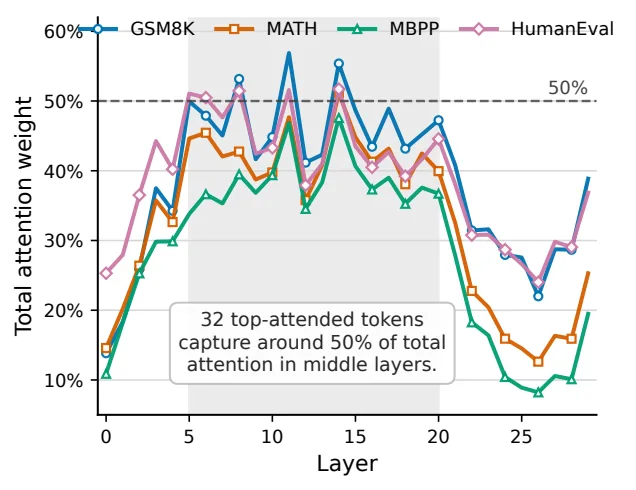
This figure shows why this example works. As in the left panel, middle layers concentrate on a few tokens, and as in the right panel, higher confidence increases per-step acceptance (source: Fig. 1b-c).
The second figure corresponds to the actual verification pipeline from draft sorting through the $\epsilon$ and $\gamma$ threshold decisions (source: Fig. 2).
Tearing Down 1 Secret Weapon
If forced to choose between the fused kernel and self-verification, choose self-verification. The kernel trims constants, while verification changes the slope (source: §3.3).
| Configuration | Accuracy | Throughput | Tokens/step | Interpretation |
|---|---|---|---|---|
| Flash-Cache + confidence-based, $B=16$ | 82.24% | 131.8 tokens/s | 2.8 tokens/step | Baseline (source: Tab. 6) |
| Flash-Cache + Flash-Verify, $B=16$ | 81.73% | 186.2 tokens/s | 5.7 tokens/step | +41.3% throughput, about 2.0× tokens/step (source: Tab. 6) |
| Flash-Cache + Flash-Verify, $B=32$ | 83.02% | 199.8 tokens/s | 5.7 tokens/step | +43.2% over confidence-based with batch scaling (source: Tab. 6) |
| Fused kernel alone, RTX 3090 | - | 1.37× per layer | - | Removes the RoPE- and cache-write-dominated region (source: Fig. 1a) |
The mechanism is clear. Confidence-based decoding discards a token from the marginal $q_i$ even when it is correct if it does not pass $\epsilon$ (source: Appx. C). Flash-Verify asks again under $p_{i_k}$ conditioned on earlier drafts. As contextual evidence accumulates, $\tilde{c}$ rises and the $r=0.48$ correlation turns into throughput (source: Fig. 1c, Fig. 6). At $\gamma=0.60$, it decodes 7.2 tokens/step with throughput similar to confidence-based decoding at 5.6 tokens/step but 3.5pp higher accuracy. As tokens/iteration grow, the accuracy gap narrows while the throughput advantage widens up to 1.33× (source: §3.3, Fig. 6).
Performance Validation: Key Results
Experimental Setup
The default is a single NVIDIA A100 80GB GPU, Triton 2.0 fused kernels, and LLaDA-1.5 evaluation (source: §3.1). Benchmarks are GSM8K 5-shot, MATH 4-shot, HumanEval 0-shot, and MBPP 3-shot, with generation lengths of 256 tokens and 512 tokens (source: §3.1, Appx. D). Default hyperparameters are $\epsilon=0.9$, $\gamma=0.8$, block size $\beta=16$, $\beta_t=80$, and $\beta_m=64$ (source: §3.1). Throughput is mean tokens/s up to the stop token under lm-eval-harness (source: Appx. D). Tokenization and the pretraining corpus follow the LLaDA-1.5 base model with no additional training or fine-tuning. The fine-tuning strategy is not applicable (source: §3.1, Abstract).
The figure above summarizes the batch-scaling experiment. Throughput rises nearly linearly up to batch size 32, Fast-dLLM OOMs at 24, and memory is lowest across the full range (source: Fig. 4).
Key Performance Metrics
- GSM8K-512: Flash-Cache + Flash-Verify ranks first in both accuracy and throughput at 83.02% accuracy and 210.6 tokens/s. That is 81.0× over greedy no-cache at 2.6 tokens/s (source: Tab. 1).
- MATH-512: 35.98%, 210.1 tokens/s, 42.0×. The highest accuracy is 37.76% from no-cache Flash-Verify (source: Tab. 1).
- HumanEval-512: 40.24%, 185.6 tokens/s, 58.0×. The highest accuracy is 42.07% from confidence-based Flash-Cache (source: Tab. 1).
- MBPP-512: 39.00%, 148.2 tokens/s, 148.2×. Greedy Flash-Cache leads in accuracy at 39.80% (source: Tab. 1).
- Scaling comparison: against dKV-Cache at 14.9 tokens/s, Fast-dLLM at 36.8 tokens/s, FreeDave at 42.8 tokens/s, and Elastic-Cache at 41.7 tokens/s, Flash-Cache + Flash-Verify reaches 210.6 tokens/s (source: Tab. 2).
- Memory: at batch size 16, about 26 GB versus about 50 GB for Fast-dLLM, about a 48% reduction. Flat preallocated cache removes padding overhead (source: §3.3, Fig. 4b).
- Masked window $\beta_m$: growing it from 16 to 96 lowers throughput, but Flash-Verify keeps a 1.4× to 1.5× lead over confidence-based decoding, with an accuracy gap of 0.2pp to 1.2pp (source: §3.3, Fig. 7).
- Generation length and prefill: both methods peak at 256 tokens and fall by about 10.5% to 12.8% at 1024 tokens. From 1-shot to 8-shot, the Flash-Verify advantage shrinks from 1.50× to 1.35×, but the absolute lead grows from 42.6 tokens/s to 78.6 tokens/s (source: Appx. F, Tab. 5).
Critical Comparison
The strongest comparison is the same-hardware rerun against Elastic-Cache and FreeDave (source: §3.1, Tab. 2). Elastic-Cache had the best baseline accuracy at 82.79% and FreeDave the best throughput at 42.8 tokens/s, but Flash-Cache + confidence-based decoding beats both at 82.87% and 149.4 tokens/s, and adding Flash-Verify pushes further to 83.02% and 210.6 tokens/s.
Conversely, in the 256-token code setting, the throughput leader is not the accuracy leader. On HumanEval-256, 39.63% versus a best of 43.29% leaves a 3.66pp gap, and on MBPP-256, 38.20% versus a best of 41.80% leaves a 3.60pp gap (source: §3.2). On math reasoning the gap is within 1.78pp, but on short code generation there is a region where aggressive parallel commits do not replace strict single-token refinement. Confidence-based decoding peaks slightly higher at about 83.4% accuracy but drops to about 131 tokens/s throughput (source: §3.3, Fig. 5b). In other words, the Pareto frontier lies farther out on the Flash-Verify side, but conservative decoding remains for a single extreme-accuracy point.
System-Level Metrics
The primary metrics are throughput in tokens/s and peak memory in GB, not latency (source: §3.3). From batch size 1 to 32, the greedy method goes from 18.5 tokens/s to 55.0 tokens/s for 2.97×, confidence-based decoding from 51.7 tokens/s to 139.5 tokens/s for 2.70×, and Flash-Verify from 56.0 tokens/s to 199.8 tokens/s for 3.57× (source: Appx. G, Tab. 6). Training FLOPs and $/1M tokens costs are not reported, nor are energy metrics. The reproduction checklist includes code release, Triton 2.0 specification, A100 80GB specification, and standard deviations over 5 seeds, but driver versions and exact full prompts rely on the appendix evaluation scripts (source: §3.1, Appx. D-E).
Our Take: Strengths, Limitations, and Why This Matters
Strengths. The authors’ claims are consistent. Cache reuse and parallel verification are not optimized separately but tied together on the same fused kernel and preallocated cache (source: §2.3). Having no external verifier matters for deployment. Unlike FlashDLM, which uses an external autoregressive verifier, and FreeDave, which uses two independent passes, there is no extra model or training (source: §4). It is also rare for a theory appendix to close a simple intuition with TV-distance guarantees (source: Appx. C).
Explicit limitations. The authors acknowledge evaluation focused on two masked diffusion LLMs and math/code structured outputs (source: Appx. A). Continuous-space diffusion, flat confidence distributions such as long-form writing or dialogue, and fixed $\gamma$ and $\beta_m$ remain unverified.
Potential limitations. First, a strong assumption. The guarantee bounds deviation from the model’s own sequential distribution, not accuracy against the data distribution (source: Appx. C, Assumption 1). Second, the parallel error of $D_t$ still relies on the confidence-based theorem $[46, Thm. 1]$. Third, cost transparency is weak. Training compute is not applicable, but inference cost and power are missing. Fourth, societal impact inherits harmful/biased generation from the base dLLMs unchanged and does not alter safety filters (source: Appx. B).
The reason it still matters is that it reframes the dLLM deployment bottleneck from FLOPs to I/O and scheduling. Holding throughput without OOM up to batch size 32 while cutting memory nearly in half can be used directly in serving-system design (source: Fig. 4, Tab. 6).
What’s Next?: Future Directions
The authors propose adaptive $\gamma$ and $\beta_m$, open-ended generation verification, and continuous-space diffusion as extensions (source: Appx. A). Three reasonable next steps are:
- Runtime confidence-statistics scheduler: instead of fixed thresholds, attach a controller that shrinks $\beta_m$ and raises $\gamma$ when prefixes are long or uncertainty is high. This can mitigate the relative slowdown from 1-shot to 8-shot in the appendix (source: Appx. F).
- Long-context and batched-serving integration: connect the block-table design to a PagedAttention-style serving stack and test pushing the saturation point beyond batch size 16. Batch size 16 already delivers about 93.2% of batch size 32, so the efficiency point is clear (source: Appx. G).
- Separate accuracy-sensitive code tasks: to close the roughly 3pp gap on 256-token code, test hybrid commits that conservatively revert only positions with high verification failure rates (source: §3.2).
Tables from the paper
Tables converted mechanically from the arXiv e-print LaTeX source. The numbers are the paper’s own and did not pass through a model.
Table 1. Accuracy and decoding efficiency of LLaDA-1.5 across different benchmarks and decoding configurations. Each cell reports accuracy (top) and throughput with speedup over greedy decoding without caching (bottom; blueblue: tokens/s, orangeorange: speedup). Bold indicates the highest accuracy in each row, while yellow!20yellow shading indicates the highest throughput.
| Benchmark | Len | Greedy No Cache | Greedy Flash-Cache | Confidence-Aware No Cache | Confidence-Aware Fast-dLLM | Confidence-Aware Elastic-Cache | Confidence-Aware Flash-Cache | Flash-Verify No Cache | Flash-Verify Flash-Cache |
|---|---|---|---|---|---|---|---|---|---|
| GSM8K (5-shot) | 256 | 80.36 { blue6.7 (orange1.0$\times$)} | 82.87 { blue56.8 (orange8.5$\times$)} | 80.44 { blue22.5 (orange3.4$\times$)} | 80.59 { blue51.2 (orange7.6$\times$)} | 81.88 { blue45.9 (orange6.9$\times$)} | 82.34 { blue144.9 (orange21.6$\times$)} | 83.62 { blue38.2 (orange5.7$\times$)} | 81.88 { blue194.9 (orange29.1$\times$)} |
| 512 | 81.35 { blue2.6 (orange1.0$\times$)} | 82.94 { blue54.8 (orange21.1$\times$)} | 81.88 { blue17.2 (orange6.6$\times$)} | 80.82 { blue36.8 (orange14.2$\times$)} | 82.79 { blue41.7 (orange16.0$\times$)} | 82.87 { blue149.4 (orange57.5$\times$)} | 82.71 { blue32.2 (orange12.4$\times$)} | 83.02 { blue210.6 (orange81.0$\times$)} | |
| MATH (4-shot) | 256 | 33.52 { blue8.5 (orange1.0$\times$)} | 37.22 { blue67.6 (orange8.0$\times$)} | 33.60 { blue22.3 (orange2.6$\times$)} | 32.74 { blue44.4 (orange5.2$\times$)} | 33.26 { blue40.6 (orange4.8$\times$)} | 36.80 { blue144.3 (orange17.0$\times$)} | 36.98 { blue38.1 (orange4.5$\times$)} | 36.56 { blue189.7 (orange22.3$\times$)} |
| 512 | 35.63 { blue5.0 (orange1.0$\times$)} | 37.40 { blue66.2 (orange13.2$\times$)} | 35.56 { blue20.3 (orange4.1$\times$)} | 33.68 { blue44.4 (orange8.9$\times$)} | 35.84 { blue41.4 (orange8.3$\times$)} | 37.08 { blue149.9 (orange30.0$\times$)} | 37.76 { blue32.8 (orange6.6$\times$)} | 35.98 { blue210.1 (orange42.0$\times$)} | |
| HumanEval (0-shot) | 256 | 43.29 { blue7.0 (orange1.0$\times$)} | 42.68 { blue79.0 (orange11.3$\times$)} | 42.68 { blue17.5 (orange2.5$\times$)} | 34.75 { blue18.7 (orange2.7$\times$)} | 36.59 { blue20.9 (orange3.0$\times$)} | 40.85 { blue169.4 (orange24.2$\times$)} | 37.20 { blue63.2 (orange9.0$\times$)} | 39.63 { blue209.2 (orange29.9$\times$)} |
| 512 | 40.85 { blue3.2 (orange1.0$\times$)} | 41.46 { blue74.5 (orange23.3$\times$)} | 39.63 { blue9.7 (orange3.0$\times$)} | 36.59 { blue15.4 (orange4.8$\times$)} | 37.80 { blue16.8 (orange5.2$\times$)} | 42.07 { blue145.7 (orange45.5$\times$)} | 37.20 { blue57.5 (orange18.0$\times$)} | 40.24 { blue185.6 (orange58.0$\times$)} | |
| MBPP (3-shot) | 256 | 38.00 { blue2.4 (orange1.0$\times$)} | 41.20 { blue62.0 (orange25.8$\times$)} | 38.00 { blue14.2 (orange5.9$\times$)} | 34.60 { blue28.0 (orange11.7$\times$)} | 41.20 { blue32.7 (orange13.6$\times$)} | 41.80 { blue115.9 (orange48.3$\times$)} | 41.40 { blue37.7 (orange15.7$\times$)} | 38.20 { blue148.0 (orange61.7$\times$)} |
| 512 | 38.20 { blue1.0 (orange1.0$\times$)} | 39.80 { blue58.5 (orange58.5$\times$)} | 38.60 { blue11.5 (orange11.5$\times$)} | 36.20 { blue17.8 (orange17.8$\times$)} | 39.00 { blue32.8 (orange32.8$\times$)} | 40.20 { blue102.2 (orange102.2$\times$)} | 39.40 { blue31.6 (orange31.6$\times$)} | 39.00 { blue148.2 (orange148.2$\times$)} |
Table 2. Comparison of accuracy and decoding throughput across different methods.
| Metric | dKV-Cache | FlashDLM | dLLM-Cache | Dyna-dLLM | Fast-dLLM | FreeDave | Elastic-Cache | Flash-Cache (conf-aware) | Flash-Cache + Flash-Verify |
|---|---|---|---|---|---|---|---|---|---|
| Acc. (%) | 81.50 | 79.91 | 80.97 | 79.32 | 80.82 | 80.97 | 82.79 | 82.87 | 83.02 |
| TPS | blue14.9 (orange5.7$\times$) | blue15.7 (orange6.0$\times$) | blue16.8 (orange6.5$\times$) | blue38.4 (orange14.8$\times$) | blue36.8 (orange14.2$\times$) | blue42.8 (orange16.5$\times$) | blue41.7 (orange16.0$\times$) | blue149.4 (orange57.5$\times$) | blue210.6 (orange81.0$\times$) |
Table 3. The hyper-parameters of Flash-dLLM under various settings.
| Model | Benchmark | Gen Length | Tracking budget $\beta_t$ | Window size $\beta_m$ | Flash-Verify $\gamma$ | Batch size |
|---|---|---|---|---|---|---|
| LLaDA-1.5 | GSM8K (5-shot) | 256 | 64 | 64 | 0.8 | 32 |
| 512 | 64 | 64 | 0.8 | 32 | ||
| MATH (4-shot) | 256 | 64 | 64 | 0.85 | 32 | |
| 512 | 64 | 64 | 0.85 | 32 | ||
| Humaneval (0-shot) | 256 | 64 | 64 | 0.85 | 32 | |
| 512 | 64 | 64 | 0.85 | 32 | ||
| MBPP (3-shot) | 256 | 48 | 64 | 0.8 | 32 | |
| 512 | 48 | 64 | 0.8 | 32 |
Table 4. Mean accuracy (%) and throughput over five random seeds. Accuracy is shown on the first line and throughput is shown in blue on the second line. Values are mean $\pm$ standard deviation.
| $\gamma$ | Track budget $\beta_t$ $48$ | Track budget $\beta_t$ $64$ | Track budget $\beta_t$ $80$ | Track budget $\beta_t$ $96$ |
|---|---|---|---|---|
| $0.60$ | 80.230.46277.801.18 | 80.760.21261.541.00 | 81.520.50248.800.70 | 81.420.41235.820.76 |
| $0.70$ | 80.740.66252.202.52 | 81.270.65234.864.94 | 82.000.36226.663.28 | 82.350.13214.782.18 |
| $0.75$ | 80.940.81235.601.36 | 82.140.47221.680.71 | 82.520.45209.761.29 | 82.560.91208.080.51 |
| $0.80$ | 81.640.54221.063.58 | 81.730.74208.402.64 | 82.150.47197.081.54 | 82.470.47196.980.84 |
| $0.85$ | 81.461.03211.320.69 | 82.710.51197.600.70 | 82.760.84187.280.75 | 83.150.17185.700.61 |
| $0.90$ | 81.550.49206.220.50 | 82.090.53192.900.75 | 82.640.41182.160.68 | 82.750.62171.860.33 |
| $1.00$ | 81.790.64165.140.83 | 82.240.43149.600.47 | 82.960.51138.280.37 | 83.410.50131.581.41 |
Table 5. Ablation of generation and prefill lengths.
| Approach | Metric | Len. 128 | Len. 256 | Len. 512 | Len. 1024 |
|---|---|---|---|---|---|
| Flash-Cache + Confidence | Accuracy | 79.03 | 82.36 | 82.24 | 82.29 |
| Throughput | blue126.7 (orange1.00$\times$) | blue140.4 (orange1.00$\times$) | blue131.8 (orange1.00$\times$) | blue125.7 (orange1.00$\times$) | |
| Tokens/step | red2.5 | red2.8 | red2.8 | red2.9 | |
| Flash-Cache + Flash-Verify | Accuracy | 79.55 | 81.90 | 81.73 | 81.72 |
| Throughput | blue174.5 (orange1.38$\times$) | blue198.4 (orange1.41$\times$) | blue186.2 (orange1.41$\times$) | blue173.0 (orange1.38$\times$) | |
| Tokens/step | red5.6 | red5.6 | red5.6 | red5.6 |
Table 6. Effect of batch size on throughput. Using LLaDA-1.5 for GSM8K-512 (5-shot). Speedup is measured relative to Flash-Cache with greedy decoding at the same batch size.
| Approach | ACC | Tok./step | Throughput B=1 | Throughput B=2 | Throughput B=4 | Throughput B=8 | Throughput B=16 | Throughput B=24 | Throughput B=32 |
|---|---|---|---|---|---|---|---|---|---|
| Flash-Cache + Greedy | 82.94 | red1.0 | { blue18.5 (orange1.0$\times$)} | { blue28.9 (orange1.0$\times$)} | { blue37.7 (orange1.0$\times$)} | { blue46.3 (orange1.0$\times$)} | { blue51.3 (orange1.0$\times$)} | { blue53.6 (orange1.0$\times$)} | { blue55.0 (orange1.0$\times$)} |
| Flash-Cache + Confidence | 82.87 | red2.8 | { blue51.7 (orange2.8$\times$)} | { blue78.0 (orange2.7$\times$)} | { blue102.4 (orange2.7$\times$)} | { blue120.5 (orange2.6$\times$)} | { blue131.8 (orange2.6$\times$)} | { blue136.4 (orange2.5$\times$)} | { blue139.5 (orange2.5$\times$)} |
| Flash-Cache + Flash-Verify | 83.02 | red5.7 | { blue56.0 (orange3.0$\times$)} | { blue90.9 (orange3.1$\times$)} | { blue131.3 (orange3.5$\times$)} | { blue164.8 (orange3.6$\times$)} | { blue186.2 (orange3.6$\times$)} | { blue195.5 (orange3.6$\times$)} | { blue199.8 (orange3.6$\times$)} |
Table 7. Example LLaDA-1.5 (without cache) — A qualitative comparison of different decoding methods.
| whiteGreedy | whiteConfident-aware | whiteFlash-Verify |
|---|---|---|
| First find the number of multiple-choice questions Amy answers correctly: 80% * 10 questions = «10*.80=8»8 questions Then find the number of true/false questions Amy answers correctly: 90% * 20 questions = «20*.90=18»18 questions Then find the number of long-answer questions Amy answers correctly: 60% * 5 questions = «50*.60=3»3 questions Then find the total points Amy gets from multiple-choice questions: 8 questions * 1 point/question = «81=8»8 points Then find the total points Amy gets from true/false questions: 18 questions * 1 point/question = «181=18»18 points Then find the total points Amy gets from long-answer questions: 3 questions * 5 points/question = «3*5=15»15 points Then add up the points from each type of question to find her total score: 8 points + 18 points + 15 points = «8+18+15=41»41 points $\boxed{41}$ redSteps: 283, Tokens: 283, Time:64.7s | First find the number of multiple-choice questions Amy answers correctly: 80% * 10 questions = «80*.10=8»8 questions Then find the number of true/false questions Amy answers correctly: 90% * 20 questions = «90*.20=18»18 questions Then find the number of long-answer questions Amy answers correctly: 60% * 5 questions = «60*.05=3»3 questions Then find the total points Amy gets from multiple-choice questions: 8 questions * 1 point/question = «81=8»8 points Then find the total points Amy gets from true/false questions: 18 questions * 1 point/question = «181=18»18 points Then find the total points Amy gets from long-answer questions: 3 questions * 5 points/question = «3*5=15»15 points Then add up the points from each type of question to find her total score: 8 points + 18 points + 15 points = «8+18+15=41»41 points $\boxed{41}$ redSteps: 66, Tokens: 277, Time: 17.2s | First find the number of multiple-choice questions Amy answers correctly: 10 questions * 80% = «100.8=8»8 questions Then find the number of true/false questions Amy answers correctly: 20 questions * 90% = «200.9=18»18 questions Then find the number of long-answer questions Amy answers correctly: 5 questions * 60% = «50.6=3»3 questions Then find the total points from the multiple-choice questions: 8 questions * 1 point/question = «81=8»8 points Then find the total points from the true/false questions: 18 questions * 1 point/question = «181=18»18 points Then find the total points from the long-answer questions: 3 questions * 5 points/question = «35=15»15 points Then add up the points from each type of question to find the total score: 8 points + 18 points + 15 points = «8+18+15=41»41 points $\boxed{41}$ redSteps: 30, Tokens: 276, Time: 13.1s |
Table 8. Example Flash-dLLM: A qualitative comparison of different decoding methods, LLaDA-1.5
| whiteGreedy | whiteConfident-aware | whiteFlash-Verify |
|---|---|---|
| Rong saves 20 coins per month, so in one year, he saves 20 * 12 = «2012=240»240 coins. Neil saves 2/5 times more coins than Rong, so he saves 20 + (2/5) * 20 = 20 + 8 = 28 coins per month. In one year, Neil saves 28 * 12 = «2812=336»336 coins. In ten years, Neil saves 336 * 10 = «336*10=3360»3360 coins. Together, Rong and Neil have 2400 + 3360 = «2400+3360=5760»5760 coins. $\boxed{5760}$ redSteps: 224, Tokens: 224, Time:15.2s | Rong saves 20 coins per month, so in one year, he saves 20 * 12 = «2012=240»240 coins. Neil saves 2/5 times more coins than Rong, so he saves 20 + (2/5) * 20 = 20 + 8 = 28 coins per month. In one year, Neil saves 28 * 12 = «2812=336»336 coins. In ten years, Neil saves 336 * 10 = «336*10=3360»3360 coins. Together, Rong and Neil have saved 240 + 3360 = «240+3360=3600»3600 coins. $\boxed{3600}$ redSteps: 73, Tokens: 222, Time: 7.8s | Rong saves 20 coins per month, so in one year, he saves 20 * 12 = «2012=240»240 coins. Neil saves 2/5 times more coins than Rong, so he saves 20 + (2/5 * 20) = 20 + 8 = 28 coins per month. In one year, Neil saves 28 * 12 = «2812=336»336 coins. In ten years, Neil saves 336 * 10 = «336*10=3360»3360 coins. Together, Rong and Neil have saved 240 + 3360 = «240+3360=3600»3600 coins. $\boxed{3600}$ redSteps: 34, Tokens: 219, Time: 5.7s |
Figures in this post are taken from the original arXiv:2609.26796 (CC BY 4.0). Only size and format were changed.
Comments