Branching on Compressed Memory: Adding Tree Reasoning to DeepSeek-V4
TL;DR Adding tree-structured speculative decoding to DeepSeek-V4-Flash yields longer acceptance length and up to about 18.5% higher decode throughput under the same verification budget (source: §5, Fig. 4). The key is not the tree itself, but the verification-side adaptation that isolates compressed attention state per branch and commits only the accepted path (source: §4).
Core Idea
If a self-driving car predicts only a single road, it gets stuck in a dead end, but carrying an alternative through every fork improves its odds of survival. This paper does the same thing.
Linear speculative decoding has a draft model propose a single token chain and the target model verify it in one pass (source: §2.1). If the early part is wrong, the entire tail is discarded. Tree speculative decoding keeps multiple branches from a shared prefix and verifies broader candidate coverage with the same verification token budget $D$ (source: §2.1, Fig. 1).
The authors’ central hypothesis can be summarized in one sentence.
The authors assume that, by using branch-aware causal verification with ephemeral state isolation and accepted-path state refresh, they can overcome DeepSeek-V4’s online compressed-attention constraints and achieve longer acceptance length and higher throughput than the linear baseline under the same budget (source: §3, §4).
The important shift in this hypothesis is from the draft side to the verification side. While recent DSpark focused on draft efficiency and adaptive depth, this work pursues the orthogonal axis of widening verification-side width (source: §6).
Background: The Problem They Solved
Where the State of the Art Stood at Publication Time
EAGLE-3/MTP-style autoregressive speculative decoding was the standard flow, in which a lightweight draft predicts future tokens and the target verifies them in a single forward pass (source: §2.1). Tree verification itself was already an established extension in SpecInfer, EAGLE-2, Medusa, Sequoia, DySpec, and others (source: §2.1, §3).
DeepSeek-V4 was solving a different problem. It compresses online along the sequence dimension with Compressed Sparse Attention $CSA$ and Heavily Compressed Attention $HCA$, reducing storage and attention computation (source: §2.2). Unlike per-token latent KV compression, information from multiple positions is merged into a shorter, structured representation that evolves as decoding proceeds (source: §2.2).
Core Research Gap
The logical token history is still a linear sequence, but the physical attention state comes from compressed context state (source: §2.2). Linear speculation only needs to extend one tentative sequence, while a tree must verify mutually exclusive branches simultaneously. After a branch point, the compression results diverge (source: §3.2).
The three challenges stated by the authors are as follows (source: §3).
- Branch-aware causal verification and isolation: a candidate must see only its own ancestors, never other branches. Physical batch order and logical dependencies diverge (source: §3.1).
- Compressed-state consistency and accepted-path refresh: $CSA$ / $HCA$ produce different compressed tokens and intermediate buffers per branch. Verifying tokens alone is not enough; the compressed state must also match the accepted sequence (source: §3.2).
- Execution overhead and optimized-path compatibility: tree construction, metadata, ephemeral state, and accepted-path extraction add latency to every cycle. Variable tree shapes break stable-shape assumptions such as CUDA Graph replay or preallocated memory (source: §3.3).
In short, the gap was not a single tree mask, but target-verification adaptation that preserves tree semantics end to end over compressed and reorganized context (source: §3, §4).
New Approach: Three-Stage Speculative Forward with Accepted-Path Refresh
The three most original contributions can be distinguished as follows (source: §4).
- Novel application of an existing methodology + systems adaptation: a three-stage forward pass integrating EAGLE/MTP-style tree speculation into the DeepSeek-V4-Flash pipeline and SGLang. It is split into draft expansion, draft decoding, and target verification (source: §4.1, §4.4).
- New state-management mechanism: it separates token-level KV from path-dependent compressed state and introduces a scratchpad for isolated per-candidate-chain compression. It never writes directly to the persistent cache and commits only the accepted path (source: §4.2).
- New engineering insight: overhead-controlling optimizations such as the different refresh schedules of $C4$ and $C128$, device-side metadata processing, and a CUDA Graph coverage cap (source: §4.3).
The strength from the authors’ perspective is clear. In dense attention, a tree is adequately served by a mask over shared KV, but in compressed attention the state itself diverges after a branch, so verification-side isolation and refresh are mandatory (source: §6). They therefore explain the net gain as follows.
$$ \text{net gain} \approx \text{extra acceptance from width} - \text{extra verification cost from cross-branch state divergence} $$The above equation summarizes the authors’ discussion, and they view the second term as the largest one under the compression paradigm (source: §6).
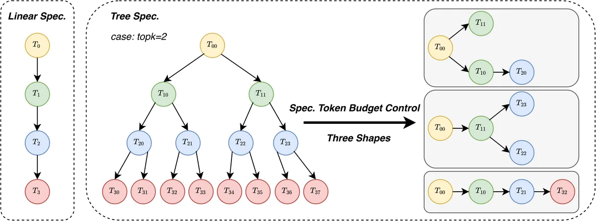
The figure above shows linear speculation following a single chain $T_0 \to T_1 \to T_2 \to T_3$, while tree speculation branches at $T_{00}$ and keeps three representative shapes through budget-controlled pruning (source: Fig. 1). The important point is that the shape itself is not fixed, but varies with draft output and budget (source: §4.1).
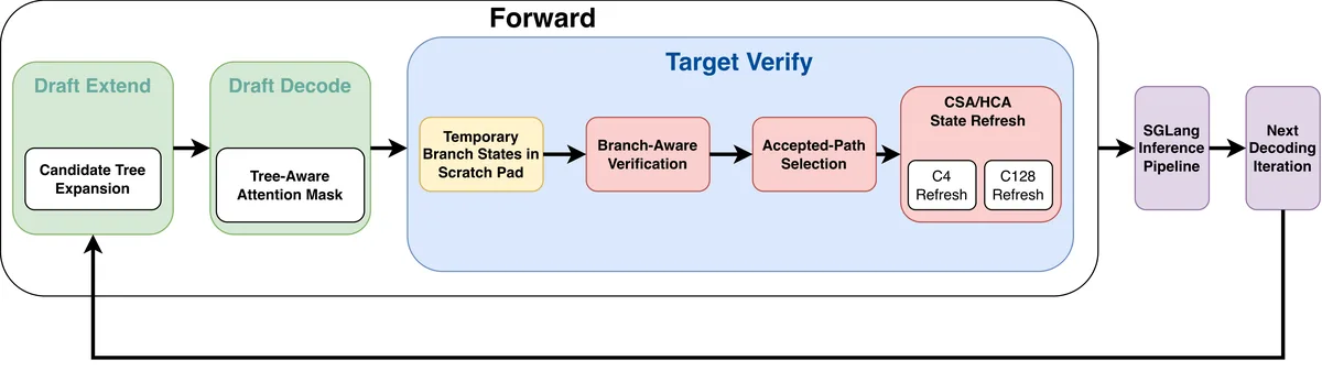
The pipeline above summarizes the SGLang integration flow (source: Fig. 2, §4.4). When the accepted prefix and persistent cache come in, it expands the candidate tree, computes candidate representations with a tree attention mask, and then defines candidate chains and compression boundaries in verification preprocessing. Mixing different chains in one compression operation would blend mutually exclusive histories, so each chain is compressed independently (source: §4.1). During verification, ephemeral results stay in the scratchpad, and after accepted-path selection only the token history and KV, the $CSA$ / $HCA$ compressed state, and the intermediate buffers are refreshed (source: §4.2).
  flowchart LR
  A[Accepted Prefix] --> B[Draft Extend]
  B --> C[Draft Decode]
  C --> D[Verify Preprocess]
  D --> E[Branch-Aware Verify]
  E --> F[Accepted-Path Selection]
  F --> G[C4/C128 State Refresh]
  G --> H[Next Iteration]
How It Works: A Concrete Example
Let us walk through the process with a toy example for graduate students. The vocabulary has only three tokens, A, B, C, and the already accepted prefix is A. The verification budget $D$ is 3 tokens, and the draft proposes top-2 over two steps.
Terminology: $D$ is the number of candidate tokens the target verifies at once, top-$k$ is the number of branches kept per step, $s$ is the number of draft steps, and acceptance length is the average number of tokens accepted per verification round (source: §5.1).
- Draft expansion: expand two options,
BandC, afterA. In the next step, expandingB, CafterBandA, BafterCmakes the full tree 1 + 2 + 4 = 7 nodes. - Budget pruning: since $D=3$, keep only the 3 top-scoring nodes. For example,
A-B,A-C, andA-B-Bremain. This is a shallow and wide tree, not a single deep and narrow chain. - Draft decoding: each candidate attends only to its own ancestral path.
A-B-BseesA, A-B, andA-Csees onlyA. The FlashMLA path of DeepSeek-V4 supports tree attention, so only layout and metadata are supplied (source: §4.1). - Verification preprocessing: unroll the tree into chains.
Chain1 = A-B-B,Chain2 = A-C. The state of prefixAis reused, but post-branch compression is separated per chain. - Target verification: the target model verifies the two chains together. In the linear case, if the second token is wrong at
A-B-?, everything after it is invalid, but in the tree case theA-Cbranch can survive. - Accepted-path commit: if
A-Cis accepted, for example, reflect only the KV and $C4$ / $C128$ compressed state ofChain2into the persistent cache, and discard the ephemeral compressed tokens and intermediate buffers ofChain1. The next iteration starts from the new prefixA-C(source: §4.2, §4.4).
Secret Weapon: Ephemeral Branch-State Isolation
If forced to pick a single key component, it is scratchpad-based isolation. $SWA$ needs only token-level KV refresh, but $CSA$ / $HCA$ require per-chain compressed tokens and intermediate results, so writing directly into a page-based KV pool entangles page allocation and ownership (source: §4.2).
The effect of tree versus linear is summarized in the table below. Values are averaged from batch size 1 to 64, in units of tokens or % (source: Tab. 1, §5.2, §5.3).
| Budget $D$ | Representative comparison | Linear acceptance length tokens | Tree acceptance length tokens | Relative acceptance gain % | Relative throughput gain % |
|---|---|---|---|---|---|
| 5 | s4_k1_d5 vs s4_k2_d5 | 2.39–2.84 | 2.67–3.15 | approx. +11.0 | approx. +3–+5 |
| 6 | s5_k1_d6 vs s4_k2_d6 | 2.39–2.84 | 2.75–3.27 | approx. +14.4 | approx. +8–+9 |
| 7 | s6_k1_d7 vs s4_k2_d7 | 2.39–2.81 | 2.81–3.36 | approx. +17.1 | approx. +9–+10 |
| 8 | s7_k1_d8 vs s5_k2_d8 | 2.39–2.84 | 2.83–3.41 | approx. +18.6 | approx. +9–+10 |
The mechanism this table describes is simple. Part of the budget maintains chain depth, and the tree wins by spending the remaining surplus on width. With a small budget there is no surplus so it is close to linear, and with a large budget width pays off (source: §5.2). Yet throughput plateaus after $D \approx 6$. Acceptance keeps growing, but the per-budget increment shrinks and growing overhead cancels it out (source: §5.3).
Performance Validation: Key Results
The experimental setup is the DeepSeek-V4-Flash model, an 8-GPU NVIDIA machine, verification budgets $D=5, 6, 7, 8$, and batch sizes 1, 2, 4, 8, 16, 32, 64 (source: §5.1). The workloads are GSM8K math reasoning with high predictability, MBPP code generation, and ShareGPT open-ended dialogue with high divergence (source: §5.1). The notation s4_k2_d5 means 4 draft steps, top-2, and a budget of 5 tokens, and at the same $D$ the linear and tree variants have the target verify the same number of tokens, making it a controlled comparison of candidate organization only (source: §5.1). The key metrics are acceptance length in tokens and decode throughput (source: §5.1).
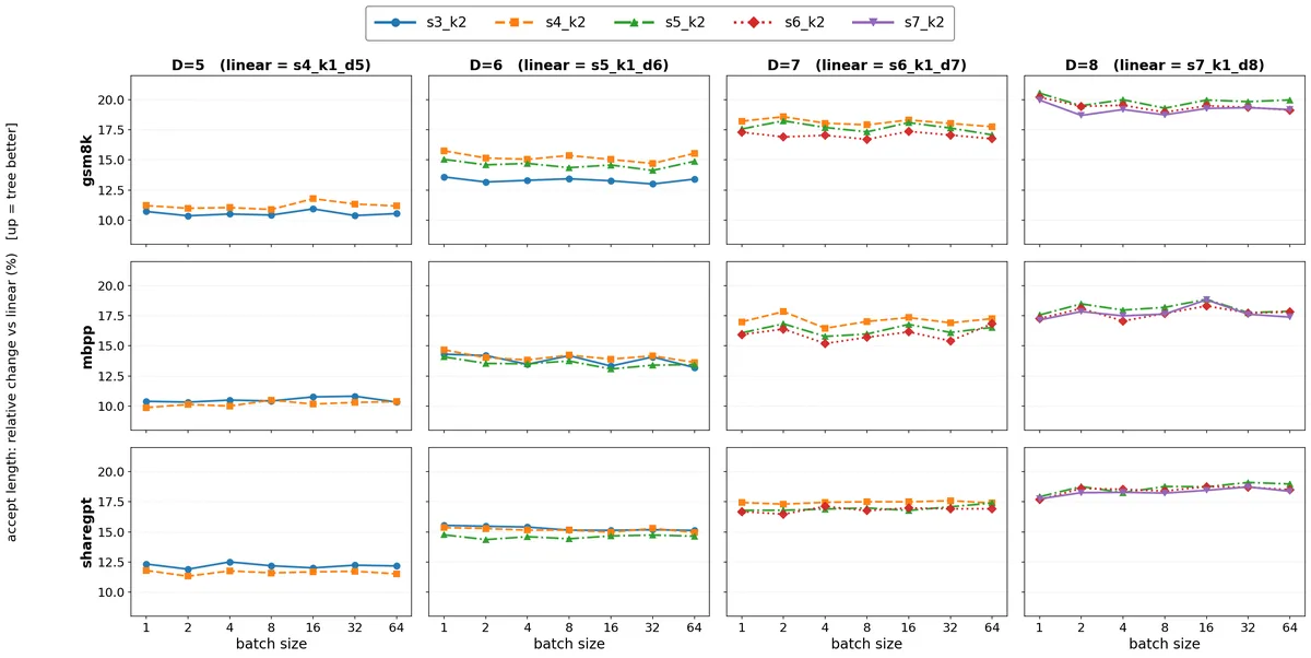
In the figure above, the tree shows higher acceptance length than linear across all budgets and batches (source: Fig. 3, §5.2). Four stable patterns stand out.
- Relative gain grows monotonically with budget: it increases from approx. +11.0% to approx. +18.6%, but the per-budget increment shrinks to approx. +3.4%, +2.6%, and +1.6%. The linear baseline stays at approx. 2.84 / 2.67 / 2.39 tokens regardless of budget (source: §5.2, Tab. 1).
- Acceptance length is nearly invariant to batch size: for a fixed configuration, variation from batch 1 to 64 is under 0.04 tokens. It depends only on draft quality and candidate structure (source: §5.2).
- Deepening the chain does not help: at the same budget, shallow-and-wide versus deep-and-narrow differ by about 2% or less. The draft’s reliable prediction horizon is the limit (source: §5.2).
- Robust across tasks: absolute values rank GSM8K, MBPP, and ShareGPT in that order, but relative gains cluster within 1–2 percentage points per budget. MBPP is the lowest, and GSM8K and ShareGPT are similar (source: §5.2).
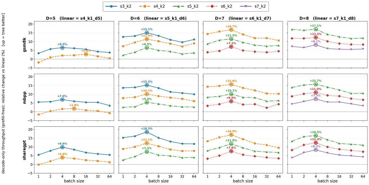
Throughput is positive in most configurations and near breakeven only at small budgets (source: Fig. 4, §5.3).
- The budget must be large enough to beat overhead: average gains plateau at approx. +3–+5% for $D=5$, approx. +8–+9% for $D=6$, and approx. +9–+10% for $D=7$–8. A case such as s4_k2_d5 at batch 1 for $D=5$ is near 0% (source: §5.3).
- At the same budget, fewer steps are better: for $D=6$, gains fall from approx. +13% for s3_k2 to approx. +9% for s4_k2 and approx. +4% for s5_k2. Since acceptance length is insensitive to steps, the difference comes from serial draft forwards and tree-width overhead (source: §5.3). Still, going too shallow leaves insufficient depth, so the optimal depth shifts with draft capability (source: §5.3).
- Batch size is an inverted U: it peaks near batch 4 and declines toward 64. For $D=6$, roughly approx. +8% at batch 1, approx. +11% at batch 4, and approx. +7% at batch 64. Since acceptance length is batch-invariant, this is a pure execution effect: verification savings dominate when memory-bound at small sizes, while candidate verification causes compute contention when compute-bound at large sizes (source: §5.3).
- The least predictable workload accelerates the most: ShareGPT is the highest, and the global maximum of approx. +18.5% comes from s3_k2_d6 at batch 4. Tree width recovers the most waste where a single chain fails early (source: §5.3).
From a baseline-comparison perspective, the strongest evidence is the same-budget controlled comparison. Holding the number of verified tokens equal and changing only the organization raises acceptance length across the board and raises throughput in most cases (source: §5.2, §5.3). Conversely, the points of marginal improvement are also clear. At small $D=5$ budgets, deep-step configurations, and large batch 64, overhead eats into the gain (source: §5.3). The authors note that their general multi-GPU setup is not optimized for high-concurrency serving, which causes variation at large batches (source: §5.3).
From a systems perspective, implementation and resources are as follows. The key dependencies are the SGLang inference pipeline, DeepSeek-V4’s FlashMLA/attention path, and CUDA Graph (source: §4.1, §4.3, §4.4). Evaluation focuses on effective decoding throughput and accepted tokens per round rather than latency, and scalability is judged by throughput curves over batch size (source: §5.1, §5.3). Training FLOPs, tokenization, pretraining corpora, and similar details are outside the scope of this paper and are not reported (source: §5).
Our Take: Strengths, Limitations, and Why This Work Matters
Strengths lie in the honesty of the problem framing. It makes clear that this is not a paper that newly invented the tree, but an adaptation paper on how the verification side must be fixed under compressed context (source: §2, §6). The same-budget controlled comparison, the regularity analysis sweeping budget, batch, and dataset, and the observation that acceptance length and throughput decouple are in a form practitioners can use directly (source: §5).
The authors also state explicit limitations directly. Hardware-aware budget tuning is out of scope (source: §3.3). This is not a high-concurrency setup, so there is large-batch variation, shallower is not always better, and the optimal depth deepens as the draft gets stronger (source: §5.3). Pruning is currently dominated by cumulative scores (source: §6).
We see three potential limitations. First, there are no absolute values for serving metrics such as absolute throughput in tokens/s and TTFT/TPOT in ms, making transfer to other hardware difficult (source: §5). Second, the results come from a single 8-GPU environment, so behavior entangled with tensor or pipeline parallelism and prefix caching is unknown (source: §5.1). Third, there is no quantitative breakdown of $CSA$ / $HCA$ compression ratios and $C4$ / $C128$ refresh costs, making it hard to reproduce which overhead dominates (source: §4.3).
Even so, this work matters because the direction is shifting. The more models use compressed, sparse, and structured context representations, the more the target-verification side becomes the decisive variable among the conditions under which trees pay off (source: §6). Even with a stronger draft, the benefit of width is consumed by overhead unless verification handles trees cheaply. The observation that the compression paradigm remains even as DeepSeek-V4.1-Flash moves up to $CSA2$ and drops $HCA$ suggests this adaptation work is not a one-off (source: §6).
What Is Next?: Future Directions
The future directions proposed by the authors fall into three strands (source: §6).
- Draft-side and verification-side co-design: adaptive depth as in DSpark and verification overhead are connected through tree shape, so depth and width must be decided together (source: §6).
- Adaptive workload-aware tree formation: decide tree activation and width not only from scores but from branch depth and path structure, inter-candidate dependencies, task predictability, and runtime batch size (source: §6).
- Continued target-verification adaptation: keep evolving verification adaptation in compressed, sparse, and structured context for long-context serving scalability (source: §7).
We would add two reasonable next steps. One is an online controller for a tree on/off policy conditioned on batch size and predictability. The inverted U and the maximum ShareGPT gain already hint at it (source: §5.3). The other is a microbenchmark decomposing $C4$ / $C128$ refresh and scratchpad traffic into operators and memory movement. Only then can we tell where breakeven lies at small budgets and what causes the plateau at large budgets (source: §4.3, §5.3).
Trees are not a panacea. The budget must be large enough to afford width, depth must match draft capability, and they shine most at small and medium batches and on hard-to-predict workloads (source: §5.3). When the conditions hold, the approx. 18.5% throughput gain is evidence that branches work even on compressed memory (source: §5.3).
Tables from the paper
Tables converted mechanically from the arXiv e-print LaTeX source. The numbers are the paper’s own and did not pass through a model.
Table 1. Accepted length (absolute, averaged over batch sizes 1–64) of linear and tree-structured speculation under matched verification budgets $D$. Within each budget, the linear ($k{=}1$) and tree ($k{=}2$) configurations verify the same number of candidate tokens. Accepted length is nearly invariant to batch size (spread $<0.04$ across all tested batch sizes).
| Budget | Config. | GSM8K | MBPP | ShareGPT |
|---|---|---|---|---|
| $D{=}5$ | s4_k1_d5 (linear) | 2.836 | 2.663 | 2.389 |
| s3_k2_d5 | 3.135 | 2.943 | 2.681 | |
| s4_k2_d5 | 3.154 | 2.935 | 2.667 | |
| $D{=}6$ | s5_k1_d6 (linear) | 2.841 | 2.669 | 2.392 |
| s3_k2_d6 | 3.219 | 3.038 | 2.757 | |
| s4_k2_d6 | 3.274 | 3.044 | 2.754 | |
| s5_k2_d6 | 3.256 | 3.030 | 2.741 | |
| $D{=}7$ | s6_k1_d7 (linear) | 2.845 | 2.672 | 2.392 |
| s4_k2_d7 | 3.361 | 3.129 | 2.809 | |
| s5_k2_d7 | 3.348 | 3.108 | 2.798 | |
| s6_k2_d7 | 3.329 | 3.098 | 2.795 | |
| $D{=}8$ | s7_k1_d8 (linear) | 2.842 | 2.678 | 2.393 |
| s5_k2_d8 | 3.406 | 3.163 | 2.839 | |
| s6_k2_d8 | 3.394 | 3.153 | 2.834 | |
| s7_k2_d8 | 3.387 | 3.153 | 2.830 |
Figures in this post are taken from the original arXiv:2609.24698 (CC BY 4.0). Only size and format were changed.
Comments