How Many Prefills and How Many Decodes Within a Power Budget: The Capacity-Power Pareto Front for PD-Disaggregated Inference
One-Line Summary (TL;DR)
This paper derives closed-form expressions for how provisioning $(n_P, n_D)$ in prefill-decode disaggregated inference determines serving capacity $\mu$ (req/s) and average power $P$ (W), and shows how to select the minimum-power configuration on the capacity-power Pareto front over candidate deployments (source: §2.2, §2.3). The key is modeling the coupling in which decode-side KV cache is shared between active decode requests and reservations for requests waiting for and running prefill, as a memory balance (source: §3.1.3, Fig. 2). Serving Qwen3-32B (32.8B params) on H200 GPUs (peak 989 TFLOP/s, 4.8 TB/s) with SGLang 0.5.9, the experiments achieve capacity errors of 1.2% (fixed length, 4096 input tokens / 256 output tokens), 3.0% (Mooncake trace), and 1.6% (Azure trace), and power errors of 2.3%, 2.7%, and 2.6% (source: §5.2, Tab. 2, Tab. 3).
Core Ideas
The proposed method is a power-aware provisioning framework combining two analytical models (source: §3).
- Serving capacity model: prefill is modeled with a compute-bound roofline and decode with a memory-bandwidth-bound roofline, with total capacity given by $\mu = \min(n_P \mu_P, n_D \mu_D)$ (source: §3.1, Tab. 1).
- Load-dependent power model: per-instance power is modeled as a capped-ramp function of normalized throughput $\tilde{\lambda}$, $p_s(\tilde{\lambda}_s)=\min(p_{0,s}+\gamma_s \tilde{\lambda}_s, p_{\text{sat},s})$ (source: §3.2).
- Discrete Pareto front: all candidate $(n_P, n_D)$ pairs are plotted on the capacity-power plane, and the set with no configuration delivering the same capacity at lower power is used as the selection criterion (source: §2.3, Fig. 1).
The central hypothesis can be stated in one sentence as follows.
The authors assume that minimum-power provisioning that analytically reconstructs the capacity-power Pareto front for PD-disaggregated inference without repeated profiling can be achieved by using a prefill compute roofline and a decode bandwidth roofline including KV-cache reservation coupling, together with a normalized-throughput-based capped-ramp power expression (source: §1, §3, §4).
Background: The Problem They Solved
Research Gap
As datacenter grid-interconnection delays and conditional interconnection become binding constraints, both efficiency in delivering required capacity at minimum power and flexibility in knowing the sustainable capacity under power cuts have become important (source: §1). LLM inference has become a sustained load in which request volume and request length grow together, and PD disaggregation, which provisions the two pools independently because prefill is compute-intensive while decode is memory-bandwidth-intensive, is widely used (source: §1).
The state of the art at publication time is summarized as follows (source: §1.1).
- Provisioning evaluation: Splitwise-, DistServe-, and BestServe-style simulation and measured throughput dominated, while hardware profiling was time-consuming and had to be repeated whenever the distribution changed (source: §1.1).
- Analytical models: DistServe and BestServe have analytical per-batch execution-time expressions, but the request rate satisfying latency SLOs still relied on simulation, and queueing-based methods used analytical expressions for prefill but measurements for decode (source: §1.1).
- Power models: Splitwise assumed power to be proportional to instance count and missed load dependence, while batch-power, kernel-power, and per-token-energy studies did not explain the aggregate power of a full PD deployment (source: §1.1).
The decisive limitation was that the coupling by which prefill reservations encroach on the decode KV-cache pool was not treated analytically, so per-deployment capacity could not be pinned down, and consequently the capacity-power tradeoff itself could not be drawn (source: §1, §3.1.3).
Identifying Originality
The three most important contributions are as follows (source: §1).
- New theoretical insight + analytical capacity model: prefill capacity and decode capacity are derived from the joint input-output length distribution and compute and memory limits, and the operating batch $B$ is solved as the unique solution of a memory-balance equation over prefill occupancy, decode occupancy, and unused fragments (source: §3.1, §4.2, Thm. 4.3).
- New load-dependent power model: prefill and decode are given separate capped linear ramps, and deployments are compared at the capacity point $\lambda=\mu$, so deployment power is computed from $(n_P, n_D)$ and the workload alone (source: §3.2, Fig. 3).
- Novel application of an existing methodology: discrete capacity-power Pareto front: the two-dimensional integer optimization (1) is reduced to search over the Pareto front, and model-versus-measurement selection agreement is evaluated with an $\epsilon=3$% $\epsilon$-Pareto criterion (source: §2.3, Appx. C).
Strengths from the Authors’ Perspective
The authors emphasize reduced reliance on empirical evaluation as a strength (source: §1, §5.2). The core argument is that parameters calibrated only on fixed lengths generalize to variable-length Mooncake and Azure workloads with only the length moments changed (source: §5.2). They also explain that a residence correction explicitly represents $Var(\ell_{out})$ and $Cov(\ell_{in},\ell_{out})$ to correct for the distortion of the active-batch average by long outputs, and that prefill queueing $t_W$ is included via a Kingman approximation to capture queueing effects (source: §4.1, §4.2).
New Approach: Analytical Power-Aware Provisioning
The full procedure is summarized in a single ComputeServingCapacity algorithm (source: Alg. 1, Appx. C).
- Prefill capacity: the FLOP demand of request $r$ is set to $F_r = 2N\ell_{in,r} + c_a L d \, \ell_{in,r}^2$, and dividing by the achieved compute rate $\pi \times \text{MFU}$ gives $t_{P,r}=a_P \ell_{in,r}+b_P \ell_{in,r}^2$ (source: §3.1.1). The reciprocal of the mean is the per-instance capacity.
Here $N$ is the parameter count (32.8B params), $L$ is 64 layers, $d$ is 8192 width, $\pi$ is 989 TFLOP/s, and MFU is 0.67 (source: Tab. 3, Appx. B.1).
Decode iteration time: for operating batch $B$ (mean active requests per iteration) and active mean context $\bar{\ell}_{ctx}$, mean memory traffic is set to $\bar{Q}=2N+\kappa B \bar{\ell}_{ctx}$ (bytes) and divided as $\bar{t}_D=\bar{Q}/(\beta \times \text{MBU})$ (source: §3.1.2). $\beta$ is 4.8 TB/s, MBU is 0.77, and $\kappa=4Lh_{kv}d_{head}$ (bytes/token) (source: Appx. B.1, Tab. 3). Calibration overheads $t_{iter}=1.00$ ms and $t_{req}=0.062$ ms are added to the intercept and slope (source: Appx. B.2).
Active-context correction: a residence correction is added to the arrival mean (source: Lem. 4.1).
- Memory balance and operating batch: the decoder token capacity $C_{tok}$ (tokens) is filled with prefill reservation occupancy plus active decode occupancy $B(\bar{\ell}_{ctx}+R)$ plus unused fragments (source: §3.1.3). $R$ is the number of reservation slots for output (tokens).
$\bar{t}_W$ is obtained from a Kingman approximation and the unique root of a cubic in $B$ is solved numerically on the interval $(0, \min(B^{max}, B^{\rho}))$ (source: §4.2, Thm. 4.3).
- Deployment capacity and power: decode capacity is obtained as $1/\mu_D = E_r[\ell_{out}-1]\bar{t}_D / B$ and combined as $\mu=\min(n_P\mu_P,n_D\mu_D)$ (source: §3.1.2). Power is computed under a uniform-splitting assumption as $P=n_P p_P(\lambda/n_P\mu_P)+n_D p_D(\lambda/n_D\mu_D^{max})$ and set to $\lambda=\mu$ for comparison (source: §3.2). $p_{0}$ is 133 W (prefill) / 448 W (decode), $\gamma$ is 566 W / 458 W, and $p_{sat}$ is 692 W / 678 W (source: Tab. 3).
Implementation and resources are as follows from a systems-paper perspective (source: §5.1, Appx. B).
- Software: SGLang 0.5.9, Mooncake KV-cache transfer backend, and round-robin dispatch (source: §5.1).
- Hardware: 1 instance per H200 GPU, with evaluated deployments from 2 instances to 8 instances (source: §5.1, §5.2).
- Metrics: serving capacity (req/s), total GPU power (W), TTFT (s), and TPOT (ms/token) (source: §5.2, §5.3).
- Compute cost detail: not training FLOPs but one analytical-expression evaluation plus one Brent root search per deployment to compute capacity, hence asymptotically lower cost than repeated simulation (source: Appx. C).
How It Works: A Concrete Example
As a toy example for a graduate student, consider an input-length distribution with equal mass on $\{2, 4\}$ tokens and outputs always of 3 tokens. $N$, $L$, and $d$ are constants and the calibrated $a_P$ and $b_P$ are assumed known (source: §3.1.1).
- Step 1 — Prefill: since $E[\ell_{in}]=3.0$ tokens and $E[\ell_{in}^2]=10.0$ tokens$^2$, $1/\mu_P = 3a_P+10b_P$ (s/req). Because the second moment enters, larger variance lowers capacity at the same mean (source: §3.1.1).
- Step 2 — Active context: since $Var(\ell_{out})=0$ tokens$^2$ and $Cov=0$ tokens$^2$, $\bar{\ell}_{ctx}=E[\ell_{in}]+E[\ell_{out}]/2=4.5$ tokens. When all outputs are identical, the residence correction is 0 tokens (source: Lem. 4.1).
- Step 3 — Memory balance: set $C_{tok}=10$ tokens and $R=1$ tokens. Ignoring prefill reservations gives $B^{max}\approx(10-{\rm unused})/5.5\approx1.5$ reqs. As prefill queueing grows, the first term grows and $B$ falls below 1.5 reqs (source: §3.1.3).
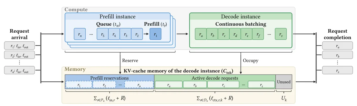
The figure above shows the KV-cache pool of a decode instance split into prefill reservations $\sum(\ell_{in}+R)$ (tokens), active requests $\sum(\ell_{ctx}+R)$ (tokens), and unused $U_k$ (tokens) (source: Fig. 2). Because request $r_1$ already reserves space in the decode pool while cycling through prefill, a backed-up prefill reduces the space available to decode, which creates the coupling (source: §3.1.3).
Secret Weapon: What Breaks Without KV-Cache Reservation Coupling
Since the paper has no direct ablation table that sets the prefill-occupancy term to 0 tokens, the qualitative effects are summarized from the mechanism and the reported numbers (source: §3.1.3, §5.2).
| Variant | $B$ (reqs) | $\mu_D$ (req/s) | $P$ (W) | Mechanism |
|---|---|---|---|---|
| Full model | $B < B^{max}$ | 1.2% to 3.0% error vs. measured | 2.3% to 2.7% error vs. measured | Prefill queueing and reservations encroach on the pool and lengthen iteration time (source: §5.2) |
| Prefill occupancy removed ($B^{max}$ used) | Overestimated | Overestimated, with larger bias especially on Mooncake (mean 8307 input tokens) | Overestimated as decode hits 678 W saturation power more often | Long inputs hold reservations for a long time, so ignoring them is fatal (source: Tab. 2, Tab. 3) |
| Residence correction removed | Under/overestimated | Larger error on traces with large $Var(\ell_{out})$ | Indirectly shifts the power reference point $\mu_D^{max}$ | Long outputs are sampled more often into the batch average (source: Lem. 4.1) |
| Kingman queueing removed ($\bar{t}_W=0$ s) | Overestimated | Capacity overestimated near the prefill bottleneck | Similar power at low load, shifted high-load branch point | Queueing diverges as $\rho_P=n_D\mu_D/n_P\mu_P$ approaches 1 (source: §4.2) |
In particular, the decode power ramp saturates at normalized throughput 0.50, creating an asymmetry in which capacity error is transmitted to power only by half, while the prefill ramp saturates at 0.99 and therefore tracks almost linearly (source: Appx. B.3).
Performance Validation: Key Results
The key metrics are mean absolute percentage error of serving capacity (req/s) and total GPU power (W), Pareto-front agreement rate, and TTFT (s) and TPOT (ms/token) upon reconfiguration (source: §5.2, §5.3). The benchmarks are not separate public benchmarks but 5 fixed-length settings (1024 tokens to 8192 input tokens, 256 output tokens) and Mooncake 1000 reqs and Azure 7200 reqs samples (source: Tab. 2, §5.1).
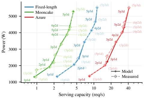
The figure above shows the modeled fronts (solid lines) closely tracking the measured fronts (dashed lines) for the fixed-length, Mooncake, and Azure workloads (source: Fig. 4). At the same power, capacity is highest for Azure, then fixed length, then Mooncake, matching the mean-input order of 1158 tokens, 4096 tokens, and 8307 tokens (source: §5.2, Tab. 2).
The results the authors emphasize most as success evidence are as follows (source: §5.2).
- Capacity generalization: 1.2% error at fixed length with 4096 input tokens, 3.0% on Mooncake, and 1.6% on Azure, generalizing outside the calibration distribution (source: §5.2).
- Power generalization: 2.3%, 2.7%, and 2.6% errors maintained with the same parameters (source: §5.2).
- Deployment-selection agreement: over 400 log-spaced required capacities, minimum-power feasible deployment choices from the model and from measurements agree in 90%, 85%, and 86% of cases, with all mismatches occurring at boundaries within 4% of measured capacity (source: §5.2, Appx. C).
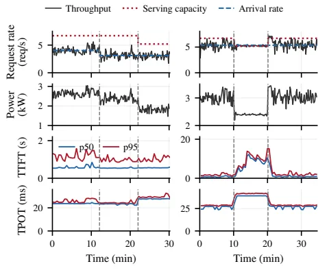
The left scenario in the figure above drops from 3p2d to 3p1d after the request rate falls to 3.1 req/s (source: Fig. 5, §5.3.1). The load drop alone reduces power by 270 W, instance removal saves an additional 560 W, median TTFT stays at 0.55 s, and median TPOT rises only from 23 ms to 28 ms (source: §5.3.1). The right scenario holds the request rate at 5.3 req/s while removing one decode for 10 min and then restoring it: 620 W is saved while capacity falls to 5.2 req/s, median TTFT rises from 0.7 s to 8.5 s, TPOT rises from 27 ms to 39 ms, and the backlog clears 1.3 min after restoration (source: §5.3.2).
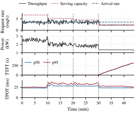
The figure above is a scale-down experiment at a fixed 3.6 req/s from 3p2d to 3p1d, 2p1d, and 1p1d (source: Appx. D, Fig. 6). The first removal saves 520 W with no TTFT change and TPOT rising only from 24 ms to 29 ms, while the second removal saves 180 W with median TTFT rising from 0.5 s to 0.9 s (source: Appx. D). The final 1p1d step has capacity 2.3 req/s, below the request rate, so TTFT diverges up to 320 s and the 470 W saving turns into the price of an unsustainable overload (source: Appx. D).
Critical Comparison
The baselines are simulation-based comparisons and measured profiling itself, with no separate SOTA scoreboard (source: §1.1, §5.2). The strongest comparison point is that minimum-power deployment selection on the Pareto front matches measurement-based selection in 85% to 90% of cases (source: §5.2). Conversely, the region with little or no improvement is the boundary band within 4% of required capacity, where model error is amplified into flipped deployment choices (source: §5.2). Mooncake, with long and highly variable inputs, also shows the largest capacity error at 3.0%, and decode power RMSE of 49 W exceeds prefill RMSE of 19 W, so power uncertainty is larger in decode-heavy deployments (source: §5.2, Appx. B.3).
Our Perspective: Strengths, Limitations, and Why This Research Matters
A strength is that combining physics-based closed forms with queueing theory means only the length moments need to be swapped when the distribution changes (source: §3, §4). In particular, the existence-and-uniqueness theorem for $B$ and the brentq numerical solution keep the implementation simple (source: Thm. 4.3, Appx. C). Closing the power expression by evaluating it at the capacity point is also a practical choice (source: §3.2).
Stated limitations are documented relatively candidly by the authors (source: Appx. B.3, §2.2).
- KV-cache transfer is assumed to overlap with prefill compute and not to be a bottleneck (source: §3.1).
- Only long-run average power is modeled, not instantaneous power; peak power is out of scope (source: §2.2).
- $t_{iter}$ and $t_{req}$ are empirical corrections without a one-to-one mapping to a specific mechanism (source: Appx. B.2).
- $c_a=2.17$ is an effective coefficient for causal-mask tile boundaries, softmax, and related effects, not an exact count for the theoretical value 2.0 (source: Appx. B.3).
- The 120 W idle power of removed instances is excluded from reported total power (source: Appx. B.3).
Potential limitations include strong assumptions such as Poisson arrivals and round-robin uniform splitting, FCFS with independent lengths, and weak correlation between iteration duration and prefill occupancy (source: §2.1, §4.2, Lem. 4.2). MFU, MBU, and the power ramps must be refit whenever the hardware, model, or serving stack changes, leaving a porting cost, and SLOs are bypassed with a $\bar{\rho}$ headroom instead of being placed directly in the constraints, leaving a gap for rigorous latency guarantees (source: §2.2, Appx. B). On societal impact, efficiency gains must be read together with operating policy because of rebound in which total demand grows instead, and because temporary capacity cuts can shift queue explosion onto user latency (source: §5.3, Appx. D).
Nevertheless, this research matters because it answers the two questions needed for grid-responsive inference, namely minimum power for required capacity and maximum capacity for a power budget, in a single picture (source: §2.3, Fig. 1). The ability to track distribution shifts without repeated simulation directly helps shorten the provisioning cycle for large fleets (source: §5.2).
What’s Next?: Future Directions
The paper concludes by presenting the analytical capacity-power relationship as a principled basis for efficient and grid-responsive operation, and does not enumerate a long separate list of future work (source: §6). Reasonable next steps in light of the limitations are as follows.
- Direct SLO coupling: replace the $\bar{\rho}$ headroom with TTFT (s) and TPOT (ms/token) distribution constraints in (1) to extend the Pareto front to a latency-constrained front (source: §2.2, §5.3).
- Heterogeneous and multi-model extension: parameterize $\pi$ (TFLOP/s) and $\beta$ (TB/s) by mixed GPU types, TP/PP parallelism, and quantization precision, while reusing the same memory balance (source: Appx. B.1, §1.1).
- Dynamic control with ESS coordination: wrap transient characteristics such as the 1.3 min queue drain after temporary cuts in model-predictive control coordinated with batteries and UPS systems to manage peaks and ramps (source: §5.3, §1.1).
- Including the transfer bottleneck: add a transfer term to the capacity expression for long-context and low-bandwidth regimes where KV-cache transfer bandwidth becomes the bottleneck (source: §3.1, Appx. B.4).
- Online recalibration: incrementally update MFU 0.67, MBU 0.77, and the power ramps as traces drift, reducing deployment flips in the boundary 4% band (source: Tab. 3, §5.2).
Tables from the paper
Tables converted mechanically from the arXiv e-print LaTeX source. The numbers are the paper’s own and did not pass through a model.
Table 1. Serving-capacity model characterization.
| Prefill | Decode | |
|---|---|---|
| resource demand | $F$ (ops) | $Q$ (bytes) |
| peak performance | $\pi$ (ops/s) | $\beta$ (bytes/s) |
| utilization | MFU | MBU |
| processing time | $t_P$ | $t_D$ |
| modeling unit | request | batch iteration |
| # requests / unit | $1$ | $B$ |
| # tokens / request | $\ell_\mathrm{in}$ | $1$ |
Table 2. Request counts and input and output lengths for the experimental workloads. The fixed-length column lists the lengths used across the fixed-length workloads; the trace columns report sample means.
| Fixed-length | Mooncake | Azure | |
|---|---|---|---|
| # requests | — | $1000$ | $7200$ |
| $\mathbb{E}_r[\ell_\mathrm{in}]$ | $1024$–$8192$ | $8307$ | $1158$ |
| $\mathbb{E}_r[\ell_\mathrm{out}]$ | $256$ | $345$ | $211$ |
Table 3. Calibrated model parameters
| Symbol | Prefill | Decode | |
|---|---|---|---|
| Serving capacity | |||
| Hardware utilization | MFU, MBU | $0.67$ | $0.77$ |
| Attention coefficient | $c_a$ | $2.17$ | |
| Per-iteration overhead | $t_\mathrm{iter}$ | $1.00$ ms | |
| Per-request overhead | $t_\mathrm{req}$ | $0.062$ ms | |
| Power ramp (W) | |||
| Static power | $p_0$ | $133$ | $448$ |
| Slope | $\gamma$ | $566$ | $458$ |
| Saturated power | $p_\mathrm{sat}$ | $692$ | $678$ |
Figures in this post are taken from the original arXiv:2609.24639 (CC BY 4.0). Only size and format were changed.
Comments